Regional Climate Dynamics

California's Sierra Nevada is a high-elevation mountain range with complex topography and significant seasonal snow cover. Anthropogenic warming in the region is expected to cause large snowpack reductions by the end of the 21st century. Locations with baseline temperatures near freezing are vulnerable to snow cover loss as warmer temperatures reduce snowfall as a fraction of precipitation (S/P) and accelerate snowmelt. Areas experiencing snow cover loss are subject to extra warming due to snow albedo feedback (SAF). SAF occurs when the disappearance of snow cover reveals lower albedo surfaces, causing an increase in absorbed solar radiation and further warming.

SAF is an important feature of climate change in snow covered regions, but climate change projections made by global climate models (GCMs) and statistical downscaling methods miss this key process. In contrast, dynamical downscaling—with a regional climate model—explicitly simulates snowpack evolution and the additional warming due to SAF. Thus, dynamical downscaling may give more plausible projections of climate change in the Sierra Nevada. The downside to dynamical downscaling is that it is very computationally expensive. Performing dynamical downscaling for an ensemble of 30+ GCMs run under multiple emissions scenarios is impractical. Instead, a statistical model is used to approximate the dynamically downscaled projections at a fraction of the cost. This approach is called hybrid downscaling. In this study, hybrid downscaling is used to create projections for all 30+ CMIP5 GCMs run under four scenarios (RCPs 2.6, 4.5, 6.0, and 8.5). First, five GCMs are selected that approximately span the range of temperature and precipitation changes in the full ensemble. These five GCMs are dynamically downscaled with the WRF regional climate model. Next, WRF output is used to build a simple statistical model called StatWRF that emulates WRF’s behavior. StatWRF is then used to downscale the entire ensemble.

One distinguishing characteristic of StatWRF is that it accounts for the warming enhancement due to SAF. Other statistical methods don’t capture this effect. StatWRF takes as input the GCM warming pattern. This is used to estimate what the downscaled warming would look like if no SAF were present—termed the background warming. To add in the additional warming resulting from SAF, StatWRF first estimates the snow cover loss resulting from the background warming, then the associated additional warming resulting from that loss of snow cover. These calculations are performed using relationships between temperature and snow cover diagnosed from the WRF simulations.

StatWRF is used to downscale warming projections (2081–2100 minus 1981–2000) from 30+ CMIP5 GCMs run under multiple scenarios. Under RCP8.5, SAF enhances the warming up to 3 °C in the late spring and early summer (Figure 1).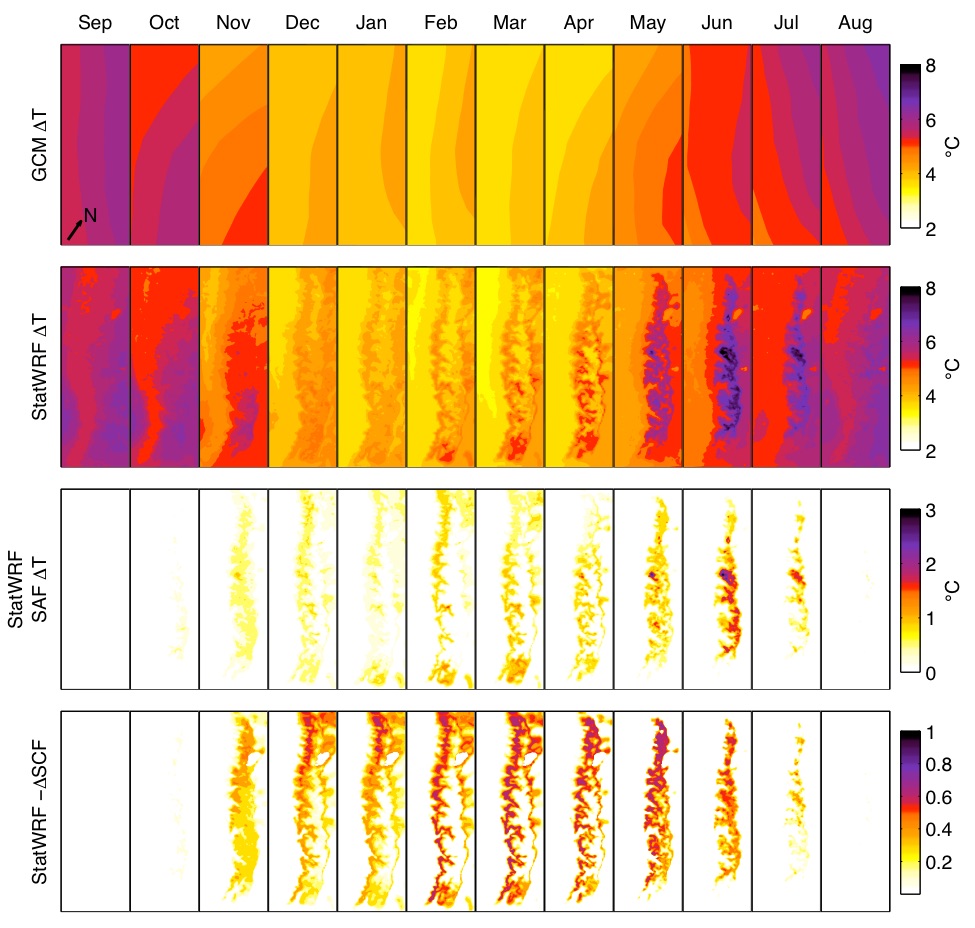

Figure 1: (Click to enlarge.) (Row 1) Linearly interpolated GCM ΔT (°C) averaged over 35 RCP8.5 GCMs for 2081–2100 minus 1981–2000. (Row 2) Same as Row 1, but StatWRF ΔT (°C). (Row 3) Same as Row 1, but StatWRF additional warming (°C) due to local SAF, which is equal to αΔSCF. (Row 4) Same as Row 1, but for StatWRF snow covered fraction loss (–ΔSCF). Grids have been rotated to vertical from their original orientation (see north arrow).

The SAF-induced warming is generally confined to an elevation band near the snow line that varies seasonally. During the middle of the snow season, from January–March, this amplification happens in roughly the 1500–3000 m elevation range (Figure 2). At the beginning and end of the snow season (October–December and May–July), the warming amplification extends from the historical snow line up to the mountain peaks. A simple calculation suggests that constraining the shortwave absorption response in CMIP5 models could reduce the ensemble-mean increase in global precipitation per unit warming at the end of the 21st century by ~20%.* Improvements in shortwave radiative transfer schemes are thus critical to attain more robust projections of the hydrologic cycle.

Figure 2: (Click to enlarge.) (left) Elevational profiles of StatWRF warming (°C). (center) WRF baseline and StatWRF future snow-covered fraction. (right) WRF baseline and StatWRF future snow-covered area (km²). Changes shown represent a downscaling of GCM climate changes between the 1981–2000 and 2081–2100 periods. The RCP8.5 ensemble mean (red line) is shown along with 25th–75th percentile (light red) and the 5th–95th percentile (pink). The ensemble-mean warming profile of the linearly interpolated RCP8.5 GCMs is shown for reference (green dashed line). For snow covered fraction and snow cover, the historical climatology is shown (black line). A bin size of 200 meters was used to create the elevational profiles. Bin midpoints are used to draw curves.

Ensemble projections for RCP8.5 with the StatWRF indicate large intermodel spread (3–5 °C) in the warming (Figure 3). However, even projections corresponding to GCMs experiencing the least warming show dramatic snow cover losses under this scenario.  Most snow cover is lost at mid-elevations (1500–3000 m), where there is substantial baseline snow cover and temperatures are close enough to freezing that warming affects S/P and snowmelt greatly.  Snow cover losses are somewhat mitigated under the lower emission scenarios, but all models predict some snow cover loss, even under the lowest scenario.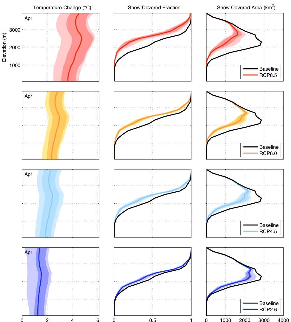

Figure 3: (Click to enlarge.) (April StatWRF elevational profiles of ΔT (left, °C), future SCF (center), and SCA (right), for RCPs 8.5, 6.0, 4.5, and 2.6. Changes shown represent a downscaling of GCM climate changes between the 1981–2000 and 2081–2100 periods. The ensemble mean is represented with dark color lines, with lighter shading marking 25th–75th percentiles, and the lightest shading marking 5th–95th percentiles. A bin size of 200 meters was used to create the elevational profiles. Bin midpoints are used to draw curves.

For more information, download the publication (Walton et al. 2017) describing these results in more detail.

Learn more about our group's research