Regional Oceanic Modeling System (ROMS)

Coastal Modeling
James C. McWilliams
Department of Atmospheric and Oceanic Sciences, UCLA
July 7, 2016
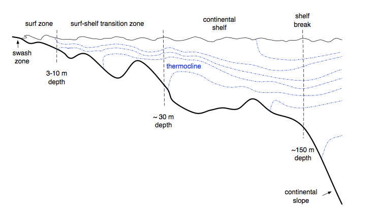
Figure 1: A sketch of a continental shelf extending from the shore through the surf zone, where surface waves break and force littoral currents, out to the upper part of the continental slope, where strong alongslope currents and mesoscale eddies are common. The outer edge of the surf zone is identified by a threshold in a/h with a the (highly variable) spectrum-peak wave amplitude and h the resting depth. It lies within the broader Surf-Shelf Transition Zone (SSTZ) that extends offshore to where the top and bottom turbulent boundary layers have separated vertically and the stable density stratification (blue dash-dot lines) is significant in shaping the vertical structure of the current and material concentrations across the rest of the shelf (e.g., outside any tidal mixing front).
1. Introduction
The coastal zone is defined here as spanning from the offshore continental slope to the shoreline as determined by averaging over the incoming waves (Fig. 1). Its physical circulation phenomena include seasonal and interannual cycles, wind-driven currents, tides, mesoscale eddies (more offshore), submesoscale density fronts and filaments, topographic wakes, internal and inertial waves, surface waves and wave-driven littoral currents, and turbulent boundary layers near the surface and bottom. It is distinctive in many ways from the deeper sea, most conspicuously in its smaller, faster scales of evolution and the greater influence of the proximate bottom in shallow water. As such, it requires special modeling techniques.
This web note is created to document our participation in the Southern California Coastal Ocean Observing System (SCCOOS) through the development of better coastal modeling techniques and the simulation of various phenomena that occur in the Southern California Bight (SCB), broadly defined. The modeling approach is with the Regional Oceanic Modeling System (ROMS), combined as necessary with the Weather Research and Forecast model (WRF) for atmospheric forcing or coupling, various surface wave models, a sediment transport module, and a biogeochemical model, although none of these companion models will be discussed here. The success of a ROMS coastal simulation depends on using a sequence of nested grids with progressively finer spatial resolution to properly convey larger-scale circulation influences and, in smaller-scale, the local coastal environment. (The same is done with regional atmospheric modeling.) Typically, our local simulations within the SCB start from a simulation of the entire U.S. West Coast, or an even larger domain.
The motivation within SCCOOS is to have a tool for coastal assessments for many particular purposes, ranging from pollution impacts, consequences of desalination and terrestrial water recapture, marine protected areas, harmful algal blooms, eutrophication, hypoxia, and climate change. We are an academic research group that publishes its results in the open literature primarily on model design and scientific discovery. Such practical management assessments have mostly lain outside our purview, although with motivation and labor our tool could be usefully applied. This note is a brief illustration of some of the simulation results to date and provides some sense of the modeling capabilities for a SCCOOS audience.
-
2. Dispersion
A common concern in the coastal environment is “fate and transport”; i.e., given the source for some anomalous material concentration or particulates, where does it go, how fast, and with what eventual outcome, including any transformation en route? In other words, dispersal, dilution, reactivity, and rising to the surface or settling to the bottom.
A simplest representation is in terms of the pair-dispersion rate. Given an ensemble of labeled fluid parcels released in close proximity, how fast does the dispersion,
D2(t) = <(x(t) - x’(t))2>, (1)
increase? Here x and x’ are separate parcel locations, and the angle brackets are an average over all parcel pairs. This rate is expressed as a Lagrangian diffusivity,
k(t) = 1 dD2 .
2 dt
(2)
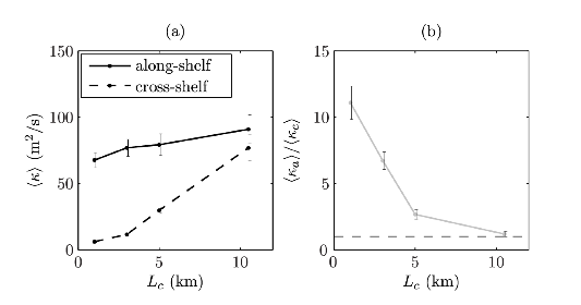
Figure 2 shows the average dispersal behavior all along the SCB nearshore region, separately for alongshore and cross-shore pair separation distances. A different dispersal questions arise for the wastewater effluent released offshore and at depth (beneath the thermocline) by the several different sewage treatment and disposal agencies along the SCB coast. Simulations made for the period of Fall 2005 are shown in Fig. 3.
Figure 2: Along- and cross-shore material relative diffusivities, ka(Lc) and kc(Lc) respectively (left panel), and their ratio (right panel) determined from particle-pair dispersion rates, averaged over ~104 pairs following nearshore releases at many sites along the shelf in the SCB. Lc is the off-shore distance of the centroid of the particle pair. ka declines only slightly with decreasing Lc within the SSTZ--indicating efficient alongshore transport even close to the shore--while kc decreases much more. Horizontal isotropy is approached with Lc ~ 10 km near the shelf break (i.e., the ratio line equal to one). This is diagnosed from realistic simulations with ROMS, except for the exclusion of surface gravity waves (i.e., without a surf zone), with horizontal grid resolutions of dx - 250 or dx = 75 m. (Romero et al., 2013)
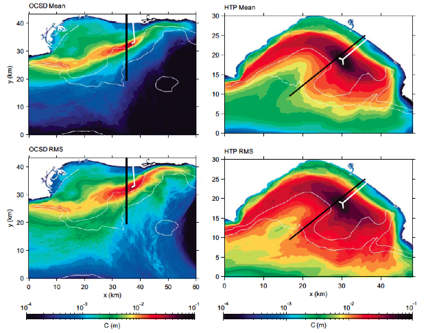
Figure 3: Time-mean and RMS values of the depth-integrated concentration of a wastewater tracer C(x.y,t) in the San Pedro Bay (left) and Santa Monica Bay (right). The model grid resolution is dx = 75 m. The tracer is defined to have unit concentration with the reported volume flux at the outfall pipes (ends of the white lines) for the Orange County Sanitation District (OCSD, left) and the Hyperion Treatment (HTP, right), with nearfield diffusers acting immediately to reduce the concentration by about a factor of 100. Instantaneous patterns of the effluent plumes show considerable submesoscale (kms) structure and variability of the continental shelves. Note that the design goal of little shoreline pollution is mostly met with these outfall pipes; similarly little effluent reaches the surface except during winter storms. However, with nearshore diversion outfalls, occasionally used for equipment repair, these design goals are often not met. See the animations of C(x,y,t) at http://www2.kobe-u.ac.up/uchiyama/sewage/
(Uchiyama et al., 2014).
A third example is the dispersal and dilution of small, seasonal river inflows and the materials they convey. Examples of this are two creeks near Santa Barbara, CA (Fig. 4), where a sequence of storms was simulated for the winters of 2005 and 2008 (Romero et al., 2016).
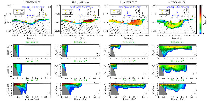
Figure 4: Evolution of river plumes from Arroyo Burro (AB, yellow circle) and Mission Creek (MC, yellow triangle) along the Santa Barbara coast during the first winter storm of 2005. Columns are four successive times during the period from 12/31/2004 to 01/02/2005 1500 (UTC). Panels a to d show surface passive tracer concentration (logarithmic base 10). The black vectors show surface currents. The inset shows the hydrographs and instantaneous discharge rates from AB (circle) and MC (triangle). The blue text and arrows show the wind speed and direction averaged over the local area. The gray dashed lines labeled s1, s2, and s3 show the positions of the vertical tracer cross-sections shown in panels (e-h), (i-l), and (m-p), respectively. The plumes spread rapidly along shore and slowly offshore, except for periods where the wind is directed offshore, and they are largely confined to the upper 5 m in depth. The horizontal grid resolution here is dx = 100 m. (Romero et al., 2016)
-
3. Shelf Fronts and Wakes
The continental shelf circulation is primarily understood to be caused by wind stress, tides, and river plumes. It is largely sheltered from mesoscale eddies that dominate the currents in deeper water. However, it does exhibit spontaneously arising submesoscale flows with horizontal scales from 100 m to 10 km. These usually take the form of either surface density fronts or filaments and their associated currents of topographic wakes generated by bottom drag near headlands or ridges that are subsequently unstable and generate coherent vortices. Such features become evident when the horizontal grid resolution of a model is fine enough, i.e., below about 1 km. These features make shelf circulations somewhat unpredictable from the wind, tide, and river forcings, and they also greatly enhance the vertical motions that transfer material concentrations across the stable density stratification profile with depth. Illustrations are in Figs. 5 and 6.
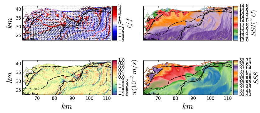
Figure 5: Ephemeral submesoscale density fronts and filaments in San Pedro Bay. (Top left) surface vertical vorticity,
normalized by the Coriolis frequency f. (Top right) Sea Surface Temperature. (Bottom left) vertical velocity w in the surface boundary layer. (Bottom right) Sea Surface Salinity. The grid resolution is dx = 75 m, and the date is Dec. 14, 2007 at 1300 PST. The black lines are bathymetric contours in meters. (Dauhajre and McWilliams, 2016)
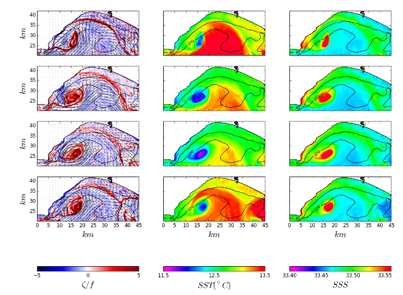
Figure 6: A sequence of snapshots of the Santa Monica Bay for (columns) normalized vertical vorticity , T, and S at the sea surface, separated in time (rows) by 8 hours, starting on Feb. 2, 2008 at 1100 (PST). A submesoscale vorticity wake is evident from the eastward flow past Pt. Dume on the left. After separating from the headland it rolls up into a coherent cyclonic vortex with a cold, salty core that indicates a net upwelling during the information event. Also evident is another submesoscale front outside Marina del Rey that forks offshore from Redondo Beach. The black lines are bathymetric contours in meters. The simulation is the same one as in Fig. 5.
-
4. Shelf-Littoral Interaction
Surface gravity waves steepen and break within the surf zone as the shoal approaching the shoreline. This generates alongshore currents through the loss of alongshore momentum from the dissipating waves, as well as sea-level set-up near the shoreline. Where the incident waves have alongshore non-uniformity, as well as where the shoreline bathymetry is non-uniform---i.e., in most realistic situations---then some of the wave-driven currents turn offshore as rip currents that are effective in cross-shore transport out over the continental shelf (including unwary swimmers).
To model this phenomenon in the context of other aspects of coastal circulation requires coupling ROMS to a surface wave model (e.g., Wave Watch III) as well as including wave-average forces and material advection in ROMS that are related to surface-wave Stokes drift. This has been done in ROMS using a wave-averaged theory (McWilliams et al., 2004) and parameterizations of wave breaking and wave-induced small-scale mixing (Uchiyama et al., 2010).
Illustrations of the simulated flow patterns and particle dispersal within Santa Monica Bay are in Figs. 7 and 8.
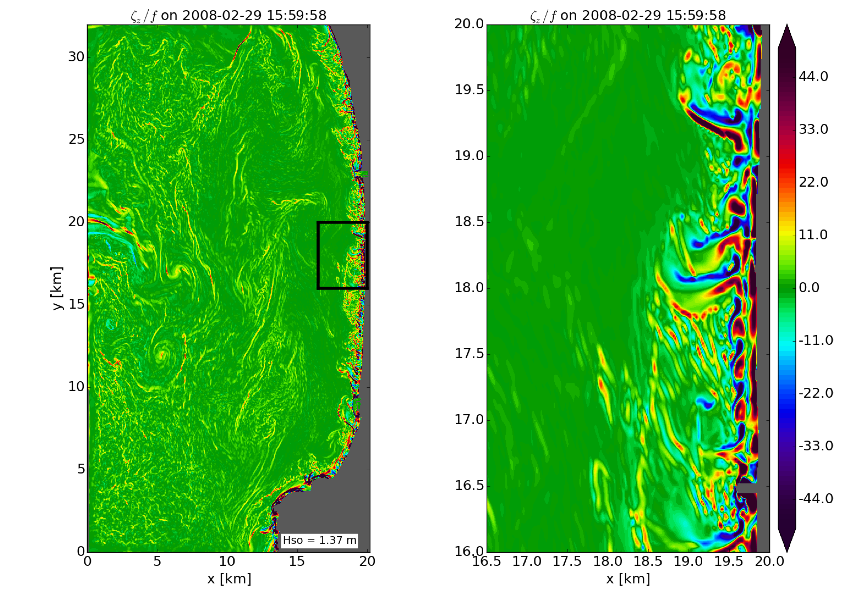
Figure 7: Surface vorticity zeta normalized by f on the shelf in Santa Monica Bay with a zoom into the littoral region off Dockweiler State Beach (black box). this is on Feb. 29, 2008, when the surface waves were relatively large for this relatively sheltered region; i.e., the significant waves height was Hs = 1.4 m. The grid resolution is dx = 20 m. Notice the frontal features on the shelf, the high vorticity in rip current patterns in the littoral zone, and intermittent ejection jets from the shoreline region into the SSTZ (Fig. 1). (Uchiyama et al., 2016)
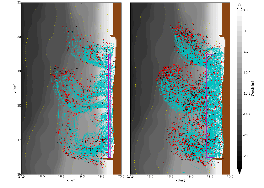
Figure 8: Particle dispersal in the littoral region in the middle of Santa Monica Bay on the same day as in Fig. 7. The particles follow 3D trajectories (turquoise lines), starting at the surface within the purple boxes in the two panesl (i.e., with the surf zone (left) and just outside (right)) and ending up 10 hours later at the positions marked with red dots. The gray scale indicates the resting depth. Notice that relatively few particles remain inside the littoral zone; instead they efficiently move out onto the continental shelf through the SSTZ (Fig. 1), often in “swarms” that indicate the organized ejection jets. (Uchiyama et al., 2016)
-
5. Prospects
With the continuing development of ROMS as a modeling tool for simulating coastal flows and their transport capacity, in particular in Southern California, we anticipate many interesting applications, both scientific and practically useful.
References
Dauhajre, D., and J.C. McWilliams, 2016: Submesoscale phenomena on the continental shelf in the southern California Bight. In preparation.
McWilliams, J.C., J.M. Restrepo, and E. M. Lane, 2004: An asymptotic theory for the interaction of waves and currents in coastal waters. J. Fluid Mech., 511, 135-178.
Romero, L.E., Y. Uchiyama, D. Siegel, J.C. McWilliams, and C. Ohlmann, 2013: Simulations of particle-pair dispersion in Southern California. J. Phys. Ocean., 43, 1862-1879.
Romero, L.E., D.A. Siegel, J.C. McWilliams, Y. Uchiyama, and C. Jones, 2016: Characterizing stormwater dispersion and dilution from small coastal streams. J. Geophys. Res., in press.
Uchiyama, Y., J.C. McWilliams, and A.F. Shchepetkin, 2010: Wave-current interaction in an oceanic circulation model with a vortex-force formalism: Application to the surf zone. Ocean Modelling, 34, 16-35.
Uchiyama, Y., E. Idica, J.C. McWilliams, and C. Akan, 2016: Wave-current interaction in Santa Monica Bay, CA. In preparation.