

 |
 |
 |
 |
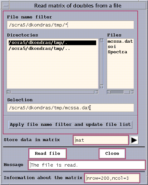
Figure 18. Read Matrix
We can plot the matrix 'mat' using the 'Matrix' function of the Plot
pull-down menu on the main window.
First, we select the name of the matrix 'mat' from the list (Fig.19), using the
arrow to the right of 'Select Matrix box in Fig 20.

Figure 19. Matrix List
and then specify the columns of the matrix to plot.
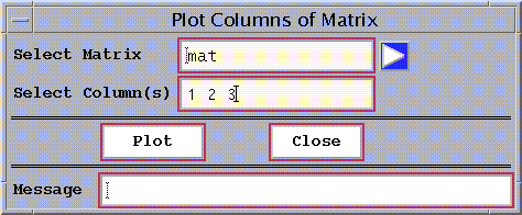
Figure 20. Plot Matrix
After pressing the Plot button, the following graphics window is launched.
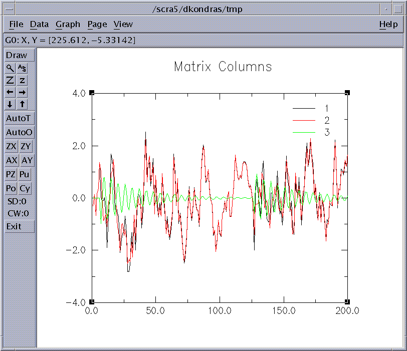
Figure 21. Test Dataset
Here the black line is the first column of the dataset - the combined data signal (see above). Our
task will be to identify weak green oscillation signal in this data.
First we use the 'Matrix/Vector' function in the 'File/Data' pull-
down menu to load the first column of
the matrix into the vector 'data'.
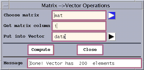
Figure 22. Matrix/Vector
Selecting the Multi-taper Method from the Analysis Tools on the main window, and after clicking Get Default Values, Compute and Plot buttons, the MTM Spectrum of the data is plotted:
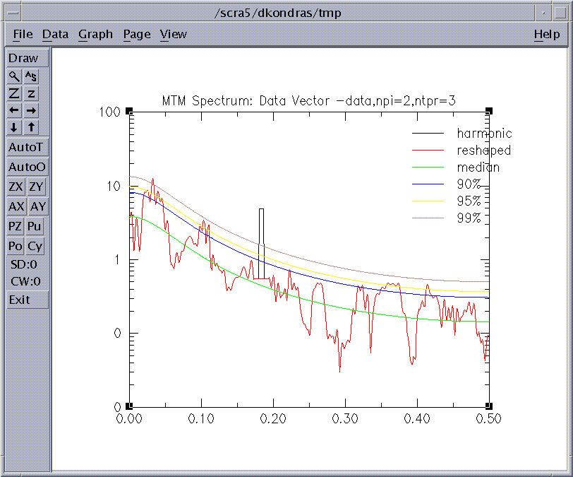
Figure 23. MTM Analysis
We see that MTM correctly isolates a significant oscillatory signal (red line ) at the correct frequency ~ f=0.18. See the MTM Demo for the details of of the MTM analysis. To confirm our findings we use the SSA analysis tool. After clicking the Get Default Values button, we change SSA window to 40, check the Strong FFT and Same Frequency pairing options in Test Options window, and then click the Compute and Plot buttons. We obtain the following SSA eigenvalue spectrum using the Error Bars significance test:
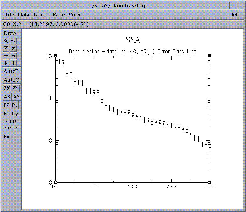
Figure 24. SSA spectrum
The pairing tests in the LogFile show that pairs 1,2 and 8,9 are candidates for oscillatory signals. To test further, we choose the Chi-squared quantitative significance test, and test against a pure red-noise null-hypothesis. We obtain the following plot:

Figure 25. SSA: Chi-Squared Test
The results of both the 'Data Eofs' and 'Null-hyp. Eofs' bases on the above plot indicate significantly elevated variance in EOFS 8 and 9, which form the pair at close to the same frequency as the weak oscillatory signal in our dataset.
As an excercise to the reader, the components with EOFS 8-9 can be reconstructed, and then passed to the MEM tool to check the frequency. Combining the results of MTM and SSA analysis, we conclude that our data contains an oscillatory signal at f=0.18.
 |
 |
 |
 |