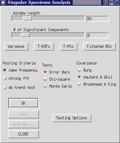
Figure 14. Singular-spectrum analysis control panel.
Clicking the `Singular Spectrum Analysis' button causes this control panel to open up:

Figure 14. Singular-spectrum analysis control panel.
There are two slide controls below the `Singular Spectrum Analysis' title.
Let us expand briefly on each of these points: (i) Commonly, SSA will use one or two low-frequency components to capture all variability that has periods greater than the window length. If there is an oscillation with a 60 month period present in a series, SSA will not be able to isolate it from other long-term fluctuations unless the window length is longer than 60 months. (ii) The number of statistically independent samples available for estimating the autocorrelation structure of a series depend (for greatest lags) on the size of the window. For example, at best (when a series has essentially no memory), only 20 samples could be used to estimate a lag-50 correlation in a time series that is 70 observations long. If the series includes memory, the number of independent samples drops quickly. Therefore Vautard et al. (1992) recommend that the window length never rise above about N/5. (iii) As a rule of thumb, SSA (and most PCA's) only seem to be able to identify on the order of M/10 significant components before oscillations start to be lumped together. Thus ideally, the window length will be somewhat greater than the longer periodicities under investigation, but also no more than about N/5 and no less than about M/10 times the number of significant components that might be present. Juggling these contraints is difficult with most real world datasets, and usually SSA results have to be judged in terms of their robustness to changes in window length. The user is therefore urged to experiment with the `Window Length' controls extensively in any Toolkit application of SSA.
As a practical matter, the choice of window length sets the dimension of the lag autocorrelation matrix to be constructed and diagonalized by SSA, and thus determines the computational burden of the application. Typically the burden is small when window length is below about 200. A slower analysis results, but is entirely feasible on most machines, with window lengths up to 1,000.
As with the other slide bars in the Toolkit, window lengths can be typed directly into the slot on the right end of the bar. The Toolkit does not expect you to conclude your entry with <enter>. Instead, as you type in the window length, the slide will move automatically to reflect your changes.
Once you have set these two controls, clicking the `OK' button will launch an SSA. Anticipating our results for the `soi' series, set the window length to 60 months and the number of significant components to 4. This window length permits us to capture the QQ El Niño oscillations while still providing a high degree of statistical significance (Keppenne and Ghil, 1992).
Make sure the "Error Bars" button under the Tests rubric is depressed (default), then click the `OK' button. The message `Working ...' appears below the slide bars, and a few moments later is replaced by `Done'. Soon thereafter a graphics window will open to display the log-eigenvalue spectrum from the specified SSA.
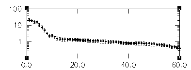
Figure 15. SSA eigenvalue spectrum for `soi'. X-axis units are SSA component
number, and y axis is variance contributed.
The eigenvalues in this spectrum are equal to the time-series variance explained by each SSA component. Since the window length was set to 60, SSA decomposes the time series into 60 components and thus 60 eigenvalues are plotted. As in many PCA's, significance of the various components can be judged qualitatively by noting which components contribute significantly more variance than would be expected from the noise background. The noise background in turn is assumed to include the components that plot in the flat-lying parts of the eigenvalue spectra, in line with the highest-order, least-contributing components. The SOI spectrum is flat-lying in the range of components from about 10 to 60. This subset probably represents the noise components. Almost certainly, they would be indistinguishable from noise by most statistical tests (see Significance tests, below).
There are 4 buttons immediately below the SSA slide bars. These buttons only should be used after the SSA `OK' button has be clicked at least once or if the program was autolaunched (that is, after SSA has been performed on the series at least once). The buttons are:
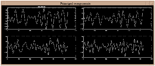
Figure 16. T-PCs plot for `soi' when 4 significant components are considered (using IDL). X-axis units are `beginning months' of the lag relations, and y axis is dimensionless SOI.
 Figure 17.
Window for selecting SSA components to be reconstructed.
Edit the list by clicking on the numbers you want to change and retyping or by clicking at the end of the list and then typing any additional component numbers. When the list is ready, click on the `OK' button to perform the reconstruction. Click the `Cancel' button to abort this action and get back to the main SSA menu.
The leading 10 components in figure 15 plot above a distinct break in the noisy part of the spectrum, and thus may contain signals that are more structured than the noise. In particular, we are interested in the leading four components which plot as two pairs of nearly equal eigenvalues: 1-2 and 3-4. As discussed earlier, pairs of nearly equal eigenvalues in SSA must be suspected of, together, capturing oscillations in the series. However, the eigenvalues plotted are subject to numerical and sampling errors (North et al., 1982), and mere pairing of eigenvalues is not enough to guarantee an oscillation has been isolated. In the eigenvalue plot above, the error bars show the ad hoc range of estimation errors that might be expected in this SSA. (See below for more sophisticated significance tests.) Any of the eigenvalues with significantly overlapping error bars could represent an "oscillatory pair'. Also eigenvalues with error bars that overlap significantly with the error bars of the noise part of the spectrum must also be suspected of being part of that noise.
The Toolkit will identify potentially paired eigenvalues among the leading S components using 3 pairing criteria which can be activated concurrently. If additional criteria are selected, the `OK' button must be clicked again with the 'Error Bars' test selected. The results of these tests are written to the log file.
For the SOI example, the log file shows that components 1-2 and 3-4 meet both criteria for being oscillations. We will return to investigate the oscillations after considering some more of the controls in the SSA part of the menu.
The final button among the paring criteria is the `Do trend Test' button in the lower lefthand part of the SSA part of the Menu. Clicking on this button prior to restarting SSA (by clicking the `OK' button) activates two tests that help to identify trending and low-frequency SSA components. The tests performed when this button is activated are:
The results of these tests are also printed into the SSA log and can be viewed by clicking the `Show Log' button in the main menu.
Choose one of the three test types, then click on the Testing Options below to set the preferences for the particular test.
dlk = (2kL/N)1/2 lk
where L is a typical decorrelation time for the time series and k is a user supplied multiplier between 1 and 2. The Toolkit estimates L to be the inverse of the logarithm of the lag-one autocorrelation of the time series. Upon clicking the `Testing Options' button, a new window will open similar to figure 18.
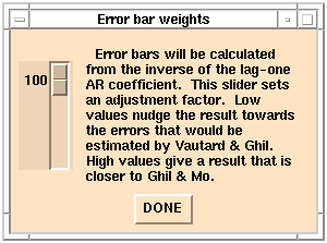 Figure 18
`Error bar weights' menu.
By dragging the slide up or down the user sets k to some value between 100 and 200 percent (1.0 and 2.0). As indicated, k values near 100 percent are closer--but not generally equal to--the liberal error bars of Vautard and Ghil (1989); k values near 200 are closer to the conservative error bars of Ghil and Mo (1991a). Click the `Done' button when a k value has been selected and the window will close so that analysis can proceed.
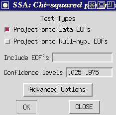 Figure 19
`Chi-Squared Preferences Panel.
All buttons have same meaning as described on the Monte Carlo SSA Preferences panel (see below), except that there are zero noise realizations by definition.
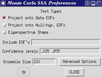 Figure 20
`MCSSA Preferences Panel.
MCSSA Test Types:
In each case, a large ensemble of red-noise surrogate time series are generated, each with the same length and same expected lag-1 autocorrelation as the time series to be tested (but see note under 'Include EOFs' below). The first two tests each use a fixed EOF basis, and can be computed individually or simultaneously by checking the individual buttons; the resulting power spectra are plotted against the dominant frequency of the EOFs in the basis. Plotting against rank will be added in a future release. The "Eigenspectrum Shape" test mutually excludes the other two, and the resulting eigenvalue spectrum is plotted against eigenvalue rank.
If no data EOFs are specified in the 'Include EOFs' slot, the null-hypothesis is pure red noise. The noise covariance matrix is computed analytically from the estimated lag-1 autocorrelation coefficient of the test time series.
If certain EOFs are specified in the 'Include EOFs' slot, the noise parameters are estimated taking into account the presence of the "signal". The resulting 'hybrid basis' is the most reliable if you have already identified a strong signal in your data (e.g. an annual cycle), which would otherwise overwhelm the noise parameter estimation.
Example: A typical testing procedure would be as follows (i) begin by testing against pure noise and identify frequencies at which the data displays anomalously high power against this null-hypothesis; (ii) find the data EOFs which correspond to these frequencies (being data-adaptive, these will often provide a better filter for the signal than the corresponding EOFs of the noise); finally (iii) re-test including these EOFs in the null-hypothesis to check if there are other features in the spectrum which were concealed by the dominant signal . It is, of course, consistent to iterate this procedure, but beware of the problem of test multiplicity discussed in Allen and Smith (1996) section 4.2: iteration makes the test increasingly liberal, so results which are still on the margins of acceptable significance after a couple of iterations including successively more EOFs into the "signal" should be ignored.
The method for estimating the autocovariance matrix that is decomposed (diagonalized) by SSA is chosen by clicking on the `Burg' button , the `Vautard et al.' button , or the ` Broomhead &King ' button in the lower right part of the menu. As indicated in the theoretical section, Burg estimation is an iterative process based on fitting an AR model with a number of AR components equal to the SSA window length. The Burg approach in principal should involve less "power leakage" due to the finite length of the time series and should therefore improve resolution (Penland et al., 1991). However, Vautard et al. (1992) found that the Burg estimate can induce significant biases when nonstationarities and very low-frequency variations are present in the series. Thus in some cases it will be worthwhile to try the Vautard et al. method. Also, for long series (N on the order of 5,000), the Vautard et al. estimate is less computationally burdensome and thus is completed more quickly. Finally, in practice, we have found that the Vautard et al. method is more prone than is the Burg method to numerical instabilities (yielding negative eigenvalues) when pure oscillations are analyzed. Both the Burg and Vautard et al. methods impose a Toeplitz structure upon the autocovariance matrix whereas the Broomhead & King method does not. The Broomhead & King method is thus somewhat less prone to problems with nonstationary time series (Allen et al., 1992b), although the Vautard et al. method seems untroubled by all but the most extreme nonstationarities. The Toeplitz methods also impose symmetries on the EOF shapes whereas the Broomhead & King method does not. However the Toeplitz methods do appear to yield more stable results under the influence of minor perturbations of the time series (Allen and Smith,1996).
To conclude our tour of the SSA menu, clicking the `Save' or `Save As' button in the main SSA menu opens a window that prompts you for which SSA results to save and where to save them. The results saved are from the most recent invocation of SSA. The window looks like
 Figure
21. `Save SSA Results' window.
SSA results (components) that can be saved are:
Click on the slot next to one of the SSA results (components) listed on the left side of the window and type in the file name where you would like to have that result saved. Make sure the corresponding button on the far left is also clicked, and then click on the OK button to actually perform the save. The Cancel button allows you to return to the Toolkit menu without actually performing the save.
And finally, to return to our analysis of SOI, having run SSA once already above, you might want to click on one or more of the buttons described above and rerun the analysis. If you click the `Filtered RCs' button, and reconstruct the first 4 components, then the resulting series will look like the following:
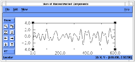
Figure 22. Reconstruction (RC) of components 1-4 of `soi'. X-axis units
are months, and y axis is dimensionless SOI units.
The series represents the sum of the results of filtering SOI by each of the 4 leading T-EOFs from SSA. The oscillatory signals are nearly all that remains. Notice, in the RC series above, the marked decrease in amplitude of the summed QQ and QB components of the SOI series between about 200 and 350 months (that is, between about 1960 and 1972). Information about these slow variations of oscillatory amplitudes typically is lost in many spectrum analyses, but is available immediately using SSA.
If this SSA-filtered RC series is now analyzed by MEM, the frequency spectrum of the RCs is much simpler than that of the complete time series, since most "noise" has been removed (Penland et al. 1991, Keppenne and Ghil 1992). Because the frequency spectrum of the series shown above is simpler, a lower-order (M=20) MEM can be applied and fewer spurious peaks result.
To do this, notice in the SSA log that the reconstructed series was save to a file called `test_rc.out'. Type this file name into the `Input file' slot at the top of the Toolkit menu and hit <enter>. Once the file has been read, click the `Maximum Entropy' button (if the MEM menu is not already open). Change the MEM Order to 10 and press th>e MEM `OK' button. The resulting spectrum should look like figure 25.
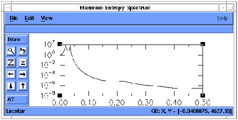
Figure 23. MEM spectrum of RC 1-4 of `soi'. X-axis units are cycles
per month, and y axis is power density.
The MEM spectrum of the RC series shows the same QQ and QB peaks as in original SOI series, but with no spurious peaks and an increase in the signal-to-noise ratio from 10 for the unfiltered to 1010 for the filtered data.The individual peaks are also more clearly defined.
Recall that the initial MEM spectrum showed peak power at 26 months and 52 months. However, at the MEM order necessary to resolve these peaks, many spurious peaks also appeared. Using SSA, the oscillations were identified instantly without having to search for some nominally optimal bandpass filter. The contributions to the original series from the leading oscillatory components were reconstructed and then passed again through the maximum-entropy analysis. The next step in such an analysis might be to use the Toolkit setting to quickly explore the sensitivity of results to various MEM orders and SSA window lengths.
MTM analysis of the RCs of components 1-4 of 'soi' yields a spectrum like figure 24. Notice that the noisy high-frequency parts of the MTM spectrum have been much reduced.
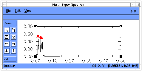
Figure 24. MTM spectrum of reconstruction of SSA components 1-4 of `soi'.
X-axis units are cycles per month, and y axis is power density.
To complete the other example, when SSA is applied to the contrived series `ssa_mstr' with a window length of 40, the eigenspectrum looks like figure 25.

Figure 25.--SSA eigenvalue spectrum for `ssa_mstr'. X-axis units are
SSA component number, and y axis is eigenvalue (or variance contributed).
SSA is clearly indicating that there are two sets of paired, non-noise components in this series, as we expect. MEM analysis of the reconstruction of those first 4 components yields the power spectrum in figure 26.The signal-to-noise ratio has been increased by 104, and the two peaks are even more clearly separated than before application of SSA.
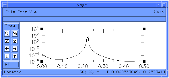
Figure 26.--MEM spectrum of RC of components 1-4 of `ssa_mstr'. X-axis
units are cycles per sample, and y axis is power density.
By now, if you have been following closely, you have seen essentially every control that the Toolkit provides, except for those that are specific to the particular graphics packages used. A close reading of some of the pertinent literature is warranted at this time. Also, `README' files are provided that outline some of the more crucial controls in the graphics packages.
Special Note---TOOLKIT FUNCTIONS IN BATCH MODE: The Toolkit's Graphical user interface is actually a front end for several FORTRAN programs that perform the actual calculations. We refer to these programs as the tools. The tools have been structured as Unix commands so that users can run them independently from the interface. They are described by Unix manual pages, now written in hypertext, and which have been included with the Toolkit. The pages describe the operation of the tools called ssa, mcssa, spectrum, carlo, and mtm (described briefly in the next section).
With some simple scripts, the user could do multiple production runs of one or more of the Toolkit functions. An example of such a script follows. This script (a) runs a user-provided program `series.read' to extract various series numbered from 1 to 30 from a large dataset and put them, in turn, into a file called `t', (b) uses the Toolkit `spectrum' tool to perform an MEM analysis on each time series in turn, (c) adds the latest MEM spectrum--in file `mem.out'--to the sum of the previous ones, and (d) then puts the sum into a file called `spectrum.all'.
#!/bin/sh
i=1
while [ "$i" -le 30 ]
do
i=`expr $i + 1` series.read<<END
$i
END
echo Using Toolkit spectrum tool to MEM series $i
spectrum t -p 40 -f 252
paste mem.out spectrum.all >! t
awk '{print $1,$2+$4}' t >! spectrum.all
done
rm t mem.out
echo End of script
---------------------------
The Toolkit provides a powerful set of tools and, like any powerful tool, provides lots of opportunities for MISAPPLICATION. Please be careful and wherever possible rely on common sense and the robustness of results more than on the simplicitty of images on the screen. Also remember that the line between noise and signal can be subjective and transitory.