|
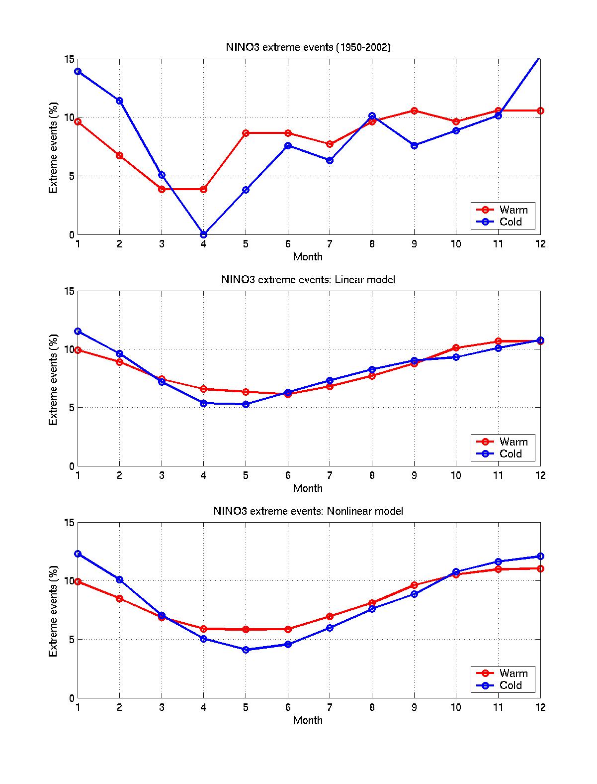
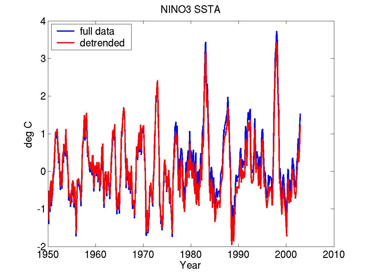
We apply a multiple polynomial regression of sea-surface temperature anomalies (SSTA) to obtain both linear and nonlinear stochastically forced models of ENSO. The 1950-2002 Kaplan extended SSTA dataset (IRI/LDEO Climate Data Library, January 1950-December 2002), 60N-30S, 30E-110W is used for both model training and validation: the models were estimated on 1950-1995 data, and verified on1996-2002 data, which includes strong 1997-1998 warm ENSO event, Fig.1. Our stochastic ENSO model is governed by the set of ordinary differential equations (ODEs) that are derived by applying multiple polynomail regression on a few leading empirical orthogonal functions (EOFs) of observationl data. A multi-layer regression procedure is employed, where the regression residual at a given level is modeled as an ODE of predictor variables at the current, and all preceding levels. The number of levels is determined so that the lag-0 covariance of the regression residual converges to a constant matrix, while its lag-1 covariance vanishes. Thus, on the last level, the regression residual is modeled by the spatially correlated white noise, representing stochastic forcing in the model. Regression models are obtained via partial least-square (PLS) cross-validation procedure; PLS finds the so-called factors, or latent variables that both capture the maximum variance in the predictor variables, and achieve high correlation with response variables. On a first regression level the principal components (PCs) of EOFs are the predictor variables, while response variables are the PC's time derivatives. On a second and the following levels, the response variables are time derivatives of the regression residuals on the preceding level. A main feature of the nonlinear model is its ability to simulate a non-Gaussian distribution of ENSO events, with warm events having larger amplitude than cold events. This property cannot be captured by a linear model, as it is demonstrated by Nino-3 ensemble statistics, see Fig.2. Each member of ensemble is a stochactic realisation of Nino-3 index of the same length as the observed data, obtained by running a model with initial conditions for January 1950. The main features of data's nonnormal PDF, such as skewness and a fatter positive tail, though smoothed by the stochastic realisations, are reproduced quite well by nonlinear model, while not by a linear model. The seasonal dependence of ENSO is demonstrated in data and model simulations in Fig.3a and Fig.3b. In both models the locking to a seasonal cycle is achived by adding a linear oscillatory forcing with a one year period on the first regression level. The extreme events distribution for data and model simulations are presented in Fig.3b. The extreme events are defined here as Nino-3 index values exceeding one standard deviation in standardized time series. Both models seem to capture data behaviour. However, such measure does not take into account the absoulte value of the event, which is done by the so-called boxplot. The boxplot statistics for each month of the year is presented in Fig.3a. For a nonlinear model the boxplot ensemble statistics is much closer to that of a real data. Both nonlinear model and observed time series exhibit similar positively skewed outliers distribution, while for linear model it is clearly symmetric. Other observed features captured by both models are stronger interannual spread and higher outlier values in winter. ReferencesKaplan, A., M. Cane, Y. Kushnir, A. Clement, M. Blumenthal, |
|
Figure 1. Time series of the observed NINO-3 SSTA from January 1950 to December 2002 and of the same dataset with a low-frequency trend removed.
Figure 2. The histogram (bars) and superimposed fitted normal density (solid line) of the detrended observed Nino-3 index, and of Nino-3 stochastic ensembles of both linear and nonlinear models. The nonlinear model captures positive skewness of the observed time series distribution, while linear model does not.

Figure 3a. Boxplots for each month of the observed Nino-3 SSTA (detrended), and of the Nino-3 stochastic ensemble for linear and nonlinear models. Points beyond the whiskers represent outliers of the distribution; both nonlinear model and observed time series exhibit similar non-symmetric positively skewed outliers population, while for linear model it is clearly symmetric. Other observed features captured by a nonlinear model include stronger interannual spread and higher outlier values in winter.
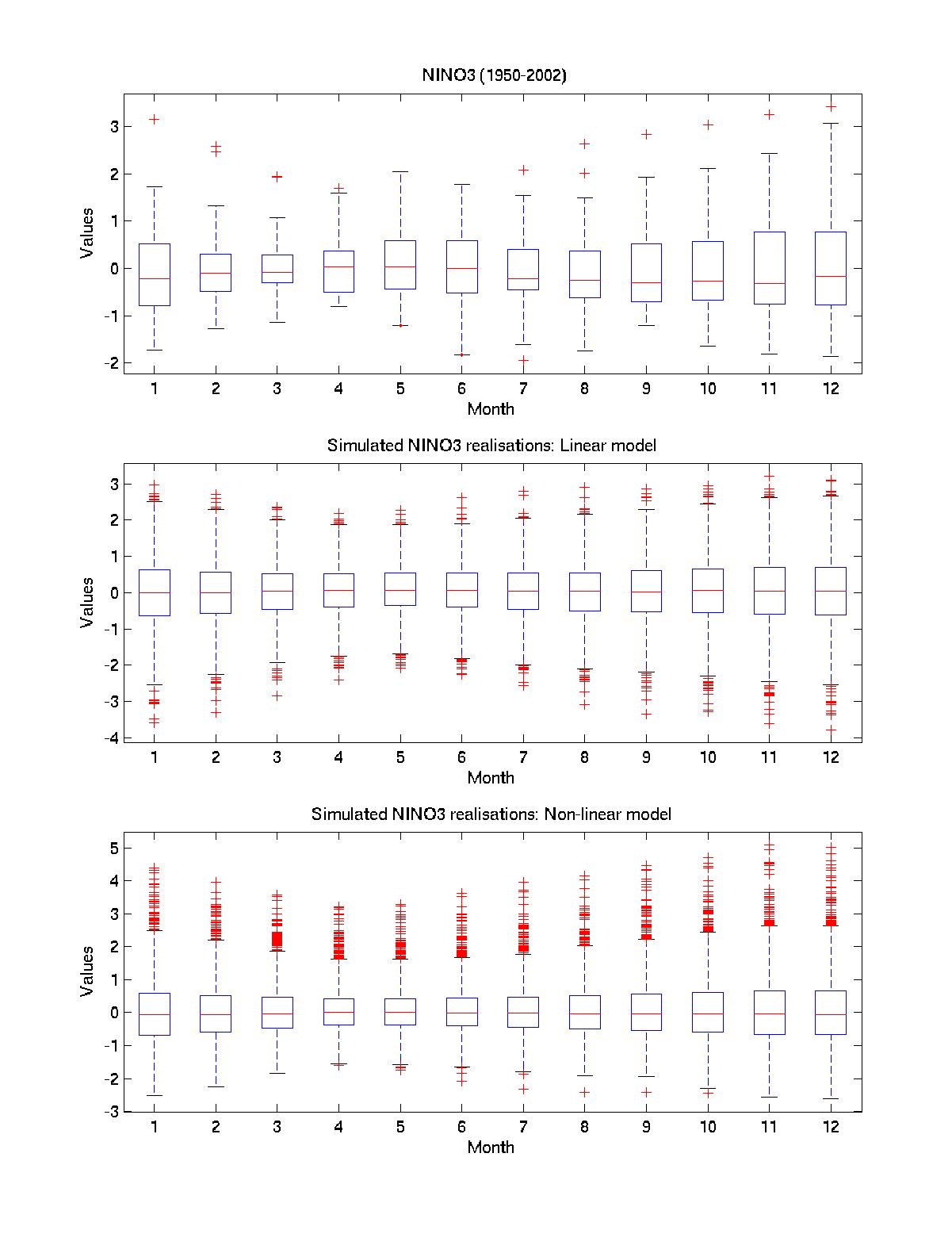
Figure 3b. Seasonal dependence of ENSO extreme events.