
 |
 |
 |
 |
As an example, we apply M-SSA to the
near-global data set of monthly
sea-surface temperatures from the Global Sea-Ice and Sea-Surface
Temperature (GISST) data set Rayner et al.-1995
for 1950-94, from 30![]() S to
60
S to
60![]() N, on a 4
N, on a 4![]() -latitude by 5
-latitude by 5![]() -longitude
grid.
-longitude
grid.
This translates into a dataset with 1295 channels, 540 months long. To read the GISST data we use the Read Matrix function from the File/Data menu on the main panel, which places the data into a matrix with a default name "mat" of 540x1295 size.
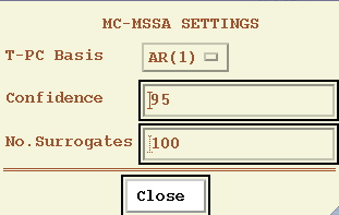
Selecting the `MSSA' option from the Analysis Tools menu on the main panel launches the following window (showing its state after pressing Get Default Values button, and specifying the parameters as described below):
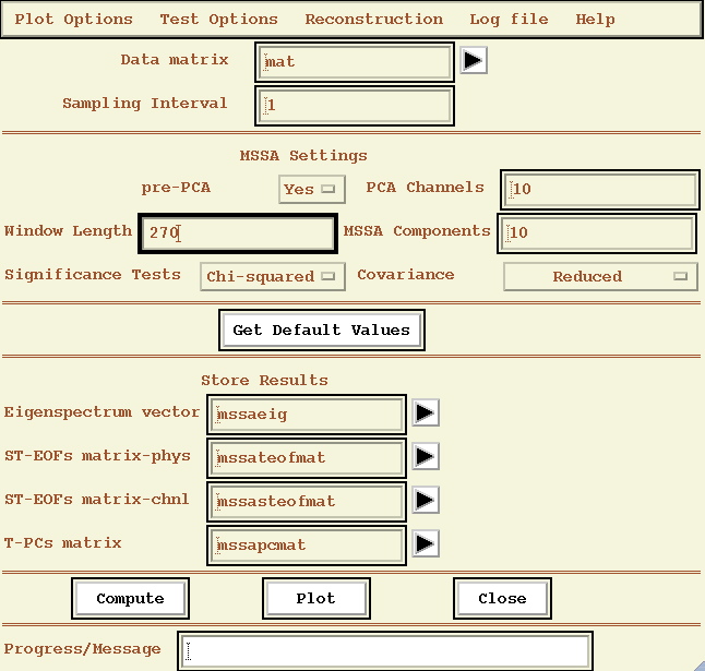
Having specified the data to be analyzed (here `mat', the GISST time-series) and the sampling interval, the principal
MSSA options to be specified are the Window Length, the type of Significance
Test, Covariance, preprocessing PCA switch, and number of PCA channels(if necessary). The number of MSSA Components
specifies how many components will be retained for future analyses. The
Get Default Values button is provided as a guide.
Note!: The value in the Window Length is taken to equal to N' if `Reduced' option is chosen for Covariance, and M for other Covariance choices.
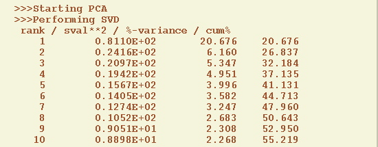
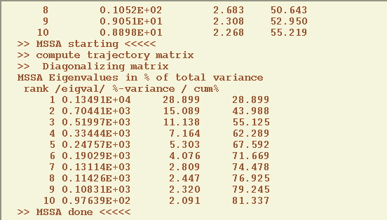
This favors the association of larger decorrelation times with larger spatial scales, as expected for climatic Fraedrich and Boettger-1978 and other geophysical fields, and the channels are uncorrelated at zero lag. After PCA the input data for MSSA has L=10 channels and length of N=540 months, and it is stored in the list of matrices as SPC; correspondent spatial EOFs are stored in a matrix SEOF
We set the Window length to 60 and 270 (N' for such option, see above).
The smaller one of M and N' determines the approximate spectral resolution 1/N' or 1/M. Choosing M=N'=270 yields the maximum spectral resolution.
The dominant frequencies of MSSA modes are computed only in Monte-Carlo or apporximate, but much faster Chi-squared MSSA test. Choosing Chi-squared in the Significance tests menu, and M=N'=270 we obtain the following plot:
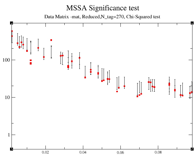
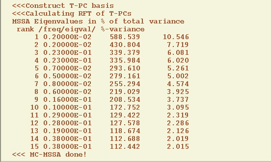
to obtain the following result:
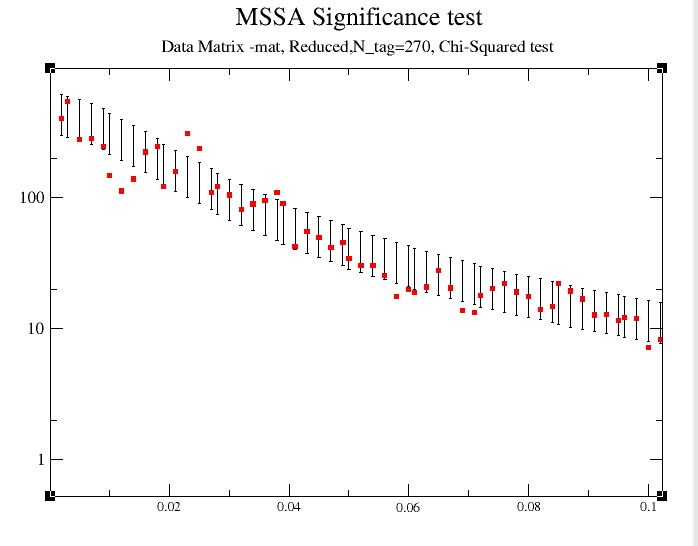
Here,
the projections are plotted against the dominant frequencies
associated with each noise eigenvector, and we have zoomed in on the 0-0.05 cy/month frequency interval of interest using the xmgr plotting tool. Since the latter are
near-sinusoidal in this case, the resulting spectrum is closely related to a
traditional Fourier power spectrum. Both the quasi-quadrennial(~0.023 cycle/month) and
the quasi-biennial(~0.038 cycle/month) modes pass the test at the 95% level (as specified in Test Options). They are well separated in
frequency by about 1/(20 months), which far exceeds the spectral resolution
of
1/M = 1/N' =
![]() .
The
two modes are thus significantly distinct from each other spectrally,
in agreement with the univariate SOI results
using MEM and MTM, respectively.
.
The
two modes are thus significantly distinct from each other spectrally,
in agreement with the univariate SOI results
using MEM and MTM, respectively.
We leave to a user to verify the above results with the Monte-Carlo test with 100 surrogates for M=N'=270, the maximum effective resolution. Computation make take a while, so be patient!
We can check that ST-EOFs of oscillatory MSSA pairs are indeed in phase quadrature using Plot Options pull-down menu:

The following plot is for a quasi-quadriennial pair 3 and 4 and channel 1:
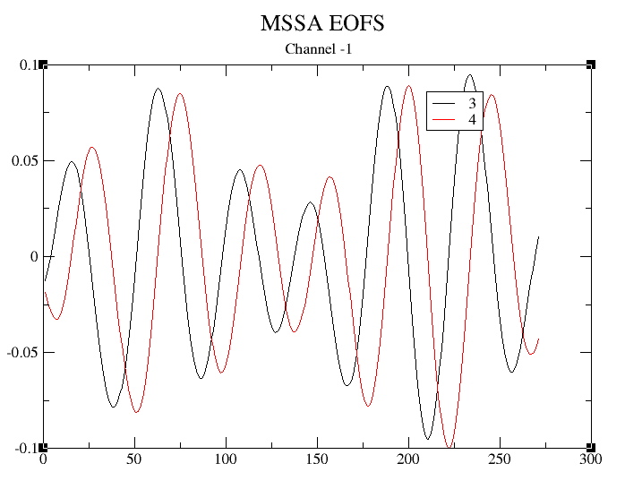
We leave as an exersise to check that a phase quadrature for a quasi-biennial pair (modes 14 and 15) is a mostly prominent for channel 2.
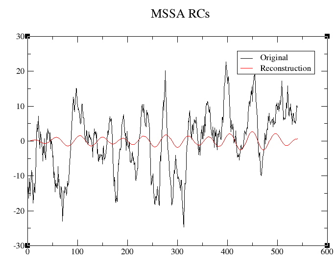
We can reconstruct the original multi-channel data or PCA components from selected MSSA modes using the Reconstruction pull-down menu in the MSSA window.
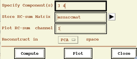
We can reconstruct either spatial PCs if PCA-prepocessing has been used or original data: choose PCA or Grid options, respectively. Here we show reconstruction in PCA space quasi-quadriennial pair for channel 1:
|
|
|
|
|