2. THEORY

e. Multi-channel Singular-Spectrum Analysis

Multi-channel SSA (or M-SSA) is a natural extension of SSA to a time series of vectors or maps, such as time-varying temperature or pressure distributions over the globe. The use of (M-)SSA for such multivariate time series was proposed theoretically, in the context of nonlinear dynamics, by Broomhead and King [1986b]. SSA can be applied in the context of systems of ordinary differential equations and the reconstruction of (the skeleton of) their attractor.

M-SSA is a generalization of this approach to systems of partial differential equations and the study of the spatio-temporal structures that characterize the behavior of solutions on their attractor Temam-1997. It has been applied to intraseasonal variability of large-scale atmospheric fields by Kimoto et al.[1991], Keppenne and Ghil[1993] and Plaut and Vautard[1994], as well as to ENSO, using both observed data Jiang et. al-1995a,Unal and Ghil-1995, and coupled GCM model simulations [Robertson et al., 1995a, b].

In the meteorological literature, extended EOF (EEOF) analysis is often assumed to be synonymous with M-SSA [Von Storch and Zwiers, 1999]. The two methods are both extensions of classical principal component analysis (PCA) [Preisendorfer, 1988] but they differ in emphasis: EEOF analysis Barnett and Hasselmann-1979,Weare and Nasstrom-1982,Lau and Chan-1985 typically utilizes a number L of spatial channels much greater than the number M of temporal lags, thus limiting the temporal and spectral information. In M-SSA, on the other hand, based on the single-channel experience , one usually chooses $L \leq M$ Often M-SSA is applied to a few leading PCA components of the spatial data, with M chosen large enough to extract detailed temporal and spectral information from the multivariate time series.

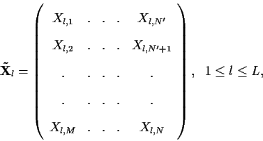
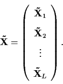
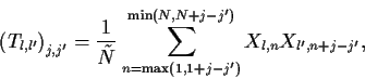
Let $\{X_{l,n}: l=1,\dots, L; n=1,\dots, N\}$ be an L-channel time series with N data points given at equally spaced intervals $n\Delta t$. We assume that each channel l of the vector ${\bf X}(t_n)$, with $t_n=n\Delta t$, is centered and stationary in the weak sense.

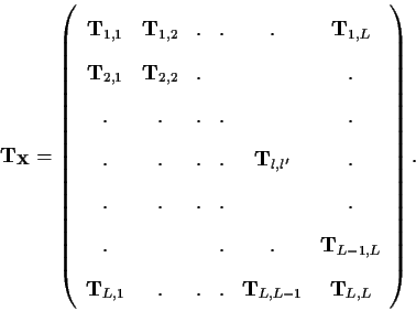
The generalization of SSA to a multivariate time series requires the constructiuon of a ``grand'' block-matrix ${\bf T}_{\bf X}$ for the covariances that has the form

$${\bf T}_{\bf X} = \left( \begin{array}{c c c c c c} {\bf T}_{... ... & . & . & {\bf T}_{L,L-1} & {\bf T}_{L,L} \end{array}\right).$$ (1)

Each block ${\bf T}_{l,l'}$ is a matrix that contains estimates of the lag covariance between channels l and l'. Extending the approach of Vautard and Ghil-1989, Plaut and Vautard-1994 proposed to obtain a ``least-biased'' estimator by using, for each lag m $(m=0,\dots, M-1)$, the longest-possible segment of each channel. Thus, the entries (j,j')of each block ${\bf T}_{l,l'}$ can be written as

$$\left(T_{l,l'}\right)_{j,j'} = \frac{1}{\tilde{N}} \sum_{n=\max(1,1+j-j')}^{\min(N,N+j-j')} X_{l,n}X_{l', n+j-j'},$$ (2)

where $\tilde{N}$ is a factor that depends on the range of summation, to wit,

$$\tilde{N}={\rm min}(N,N+j-j')-{\rm max}(1,1+j-j')+1$$ (3)

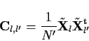
Note that, unlike in the single-channel case, here ${\bf T}_{l,l'}$ is Toeplitz but not symmetric. Its main diagonal contains the Vautard and Ghil [1989] estimate of the lag-zero covariance of channels l and l'. The diagonals in the upper-right triangle of ${\bf T}_{l,l'}$ contain the lag-m covariance of channels l and l', with l' leading l, while the diagonals in the lower-left triangle contain the covariances with l leading l'. Equation  (2) ensures that ${\bf T}_{l',l}=({\bf T}_{l,l'})^{\rm t}$ so that ${\bf T}_{\bf X}$ is symmetric, but it is not Toeplitz. Note that the original formula in Plaut and Vautard [1994]--their Eq. (2.5)--does not, in fact, yield a symmetric matrix. More generally, we only expect to obtain a grand matrix ${\bf T}_{\bf X}$ that is both symmetric and of Toeplitz form provided the spatial field being analyzed is statistically homogeneous, i.e., its statistics are invariant with respect to arbitrary translations and rotations.

An alternative approach [Broomhead and King, 1986a, b; Allen and Robertson, 1996] to computing the lagged cross-covariances is to form the multi-channel trajectory matrix ${\bf\tilde X}$ by first augmenting each channel $\{X_{l,n}:n=1, \dots, N\}, 1 \leq l \leq L$, of ${\bf X}$ with M lagged copies of itself,

$${\bf\tilde X}_{l} = \left( \begin{array}{c c c c c } {X}_{l,1... ... & . & {X}_{l,N}\\ \end{array}\right), \; \; 1 \leq l \leq L,$$ (4)

and then forming the full augmented trajectory matrix:

$${\bf\tilde X} = \left( \begin{array}{c} {\bf\tilde X}_{1}\\ ... ... X}_{2}\\ \vdots \\ {\bf\tilde X}_{L}\\ \end{array}\right).$$ (5)

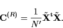
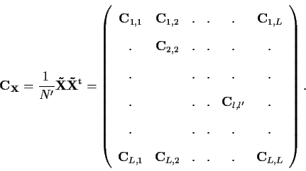
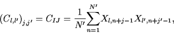
Thereafter, one computes the grand covariance matrix ${\bf C}_{\bf X}$ as

$${\bf C}_{\bf X} = \frac{1}{N'} {\bf\tilde X} {\bf\tilde X}^{\... ...bf C}_{L,2} & . & . & . & {\bf C}_{L,L}\\ \end{array}\right).$$ (6)

The blocks of ${\bf C}_{\bf X}$ are given by

$${\bf C}_{l,l'} =\frac{1}{N'} \tilde {\bf X}_{l} \tilde {\bf X}^{\rm t}_{l'}$$ (7)

with entries

$$\left(C_{l,l'}\right)_{j,j'} =C_{IJ} ={1\over N'}{\sum^{N'}_{n=1}}X_{l,n+j-1}X_{l',n+j'-1},$$ (8)

where I=j+M(l-1) and J=j'+M(l'-1) Allenand Robertson-1996. Here ${\bf C}_{l,l'}$ is neither Toeplitz nor symmetric, but again ${\bf C}_{l',l}=({\bf C}_{l,l'})^{\rm t}$ and hence ${\bf C}_{\bf X}$ is symmetric.

Each block ${\bf C}_{l',l}$ contains, like ${\bf T}_{l,l'}$ in Eq. (1), an estimate of the lag covariances of the two channels l and l'. The difference between the Toeplitz method of Vautard and Ghil [1989] and the trajectory-matrix method of Broomhead and King [1986a, b] in estimating the lag-covariance matrix, when applied to M-SSA, consists in calculating Eqs. (1) and (2) vs. Eqs. (6)-(8). The Toeplitz method extracts, according to the fixed lag m that is being considered at the moment, the two longest matching segments from the two channels l and l'; the matching is determined by the requirement that, for each entry in the designated trailing channel, there exist an entry in the designated leading channel that is m time steps ``ahead." It then uses the same estimated lag covariance for all entries along the appropriate diagnoal in the block and thus yields a Toeplitz-form submatrix.

The trajectory-matrix method gradually slides, regardless of m, the same N'-long windows over the two channels. To compute the first entry in the diagonal that contains the lag-m covariances, the two matching windows are situated so that one starts at the first time point of the trailing channel and at the (m+1)st point of the leading channel. Both windows are then slid forward by one point in time to produce the second entry. This results in slightly different values, from entry to entry, until the last point of the leading channel is covered and the (M-m)th entry of the diagonal, which is the last one, is calculated. This latter method thus retains detailed information on the variation of the lag-covariance estimates from one pair of segments of the channels l and l' to another, while the Toeplitz method produces a single, and smoother, global estimate for each lag m.

Diagonalizing the $LM\times LM$ matrix ${\bf C_X}$ or ${\bf T_X}$yields LM eigenvectors $\{ {\bf E}^{k}: 1 < k \leq LM \}$ that are not necessarily distinct. The extent to which the eigenpairs $\left(\lambda_k, {\bf E}^k\right)$ obtained by diagonalizing ${\bf C}_{\bf X}$ equal those obtained from ${\bf T}_{\bf X}$ is a good indication of the robustness of the M-SSA results. Each eigenvector ${\bf E}^{k}$ is composed of L consecutive M-long segments, with its elements denoted by E^k_l,m. The associated space-time PCs ${\bf A}^k$ are single-channel time series that are computed by projecting ${\bf\tilde X}$ onto the EOFs:

$$A^k_n = \sum_{m=1}^M \sum_{l=1}^L X_{l,n+m} E^k_{l,m},$$ (9)

where n varies from 1 to N'.

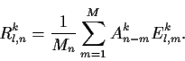
For a given set of indices ${\cal K}$, RCs are obtained by convolving the corresponding PCs with the EOFs. Thus, the kth RC at time nfor channel l is given by:

$$R^k_{l,n} = \frac{1}{M_n} \sum_{m=1}^{M} A^k_{n-m} E^k_{l,m}.$$ (10)

The normalization factor M_n equals M, except near the ends of the time series, and the sum of all the RCs recovers the original time series Plaut and Vautard-1994, as it does in the single-channel case.

Both SSA (L=1) and conventional PCA (M=1) analysis are special cases of EEOF or M-SSA analysis. Following Allen and Robertson [1996], both algorithms can be understood in practice in terms of a ``window."

These windows are illustrated schematically in the Fig.1

The axes are spatial coordinate (or spatial PC label) x, time t, and lag s; discrete values of these variables are labeled by l, n, and j, respectively (courtesy of K.-C. Mo).

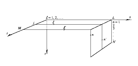
Standard PCA slides a flat and narrow window, of length 1 and width L, over the data set's N fields, each of which contains L data points. PCA thus identifies the spatial patterns, i.e., the EOFs, which account for a high proportion of the variance in the N views of the data set thus obtained. Equivalently, PCA can be described as sliding a long and narrow, $N \times 1$ window across the Linput channels and identifying high-variance temporal patterns, i.e. the PCs, in the corresponding L views. In Fig.1, the former view of things corresponds to sliding the $1\times L$ window parallel to the x-axis along the t-axis. In the latter view, one slides an $N \times 1$window that starts out by lying along the t-axis parallel to the x-axis. This latter case is also somewhat analogous to the trajectory-matrix version of single-channel SSA, except that in SSA we reduce the length of this long and narrow window to M, and consider only one channel.

These two different window interpretations carry over into M-SSA. In the first case one proceeds from spatial PCA to EEOFs. To do so, we extend our $1\times L$ window by M lags to form an $M\times L$ window that lies in the horizontal (x,s)-plane of Fig.1. By moving this window along the t-axis, we search for spatio-temporal patterns, i.e. the EEOFs, that maximize the variance in the N'=N-M+1overlapping views of the time series thus obtained. The EEOFs are the eigenvectors of the $LM\times LM$ lag-covariance matrix given by Eqs. (6)-(8).

The second conceptual route leads from single-channel SSA to M-SSA. To follow this route, we reduce the length of the $N \times 1$ window to $N'\times 1$. This window still lies initially along the t-axis and we search for temporal patterns, i.e. the N'-long PCs, that maximize the variance in the $M\times L$ views of the time series Allen and Robertson-1996,Robertson-1996. This is equivalent to SSA of the univariate time series formed by stringing together all the channels of the original multi-channel time series end-to-end, with the complementary window N' playing the role of M in SSA. The (reduced) PCs are the eigenvectors of the $N'\times N'$ reduced covariance matrix with the elements 1

$$C^{(R)}_{IJ}={1\over L}{\sum^{L}_{l=1}}\left[{\sum^{M}_{j=1}}X_{l,I+j-1}X_{l,J+j'-1}\right].$$ (11)

1

This matrix, unlike the $LM\times LM$ matrix of Eq. (6), is given by 1

$${\bf C}^{(R)} =\frac{1}{N'} \tilde{\bf X}^{{\rm t}}\tilde{\bf X}.$$ (12)

1 In typical climate applications, N'<LM; hence ${\bf {C}}^{(R)}$ is smaller than ${\bf C}_{\bf X}$ and the latter has a null space of dimension LM-N'. The eigenvectors of ${\bf C}_{\bf X}$ that lie outside this null space, i.e., that correspond to nonzero eigenvalues, are identical to those of ${\bf {C}}^{(R)}$.

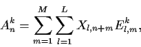
As in the single-channel case, a test of statistical significance is needed to avoid spatially smooth-looking but spurious oscillations that might arise from M-SSA of finitely sampled noise processes. The complementary N'-window approach of Eq. (11) allows the univariate SSA Monte Carlo test of Allen-1992 to be extended to M-SSA in a straightforward manner, provided ML > N', so that the reduced covariance matrix is completely determined and has full rank. N' can always be chosen sufficiently small, so that the complementary window N' used in Eq. (11) determines the spectral resolution.

Details of this essentially univariate test are given in Allen and Robertson-1996. The usefulness of the test depends in an essential way on the channels being uncorrelated at zero lag or very nearly so. In the example at hand, the decorrelation condition holds exactly, since we use the PCs of spatial EOF analysis. When using time series from grid points that are sufficiently far from each other for decorrelation to be near-perfect, the test can still be useful.

In this test, the data series together with a large ensemble of red-noise surrogates are projected onto the eigenmodes of the reduced covariance matrix of either the data or the noise. The statistical significance of the projections is estimated as in the single-channel test. The noise surrogates are constructed to consist of univariate AR(1) segments, one per channel, that match the data in autocovariance at lag 0 and lag 1, channel-by-channel. The reason an essentially univariate test can be applied is because the eigenmodes do not depend on cross-channel lag-covariance, provided N' is interpreted as the spectral window used in Eq. (11).

Varimax Rotation

The EOFs rotation has been introduced orginally as modification of standard PCA.
Spatial orthogonality of EOFs and temporal orthogonality of PCs coming from PCA impose certain limits on physical interpretability. This is because physical processes are not independent, and therefore physical modes are expected in general to be non-orthogonal. To help overcome these difficulties and gain easy interpretation, a number of methods have been proposed.

Method based simply on rotating the EOF patterns, seems to be the most widely used because of its relative simplicity. The method attempts to rotate a fixed number of EOF patterns using typically an orthogonal rotation matrix subject to maximizing given simplicity criterion. The EOFs can be either unscaled or scaled by the square root of the associated eigenvalues. The most well-known and used rotation algorithm is the VARIMAX criterion that attempts to simplify the structure of the EOFs patterns by pushing the EOF coefficients towards zero, or ±1.

Recently, Groth and Ghil (2011) have demonstrated that a classical M-SSA analysis suffers from a degeneracy problem, with eigenvectors not well separating between distinct oscillations when the corresponding eigenvalues are similar in size. This problem is a shortcoming of principal component analysis in general, not just of M-SSA in particular. In order to reduce mixture effects and to improve the physical interpretation, Groth and Ghil (2011) have proposed a subsequent varimax rotation of the ST-EOFs. To avoid a loss of spectral properties (Plaut and Vautard 1994), they have introduced a slight modification of the common varimax rotation that takes the spatio-temporal structure of ST-EOFs into account.