

 |
 |
 |
 |
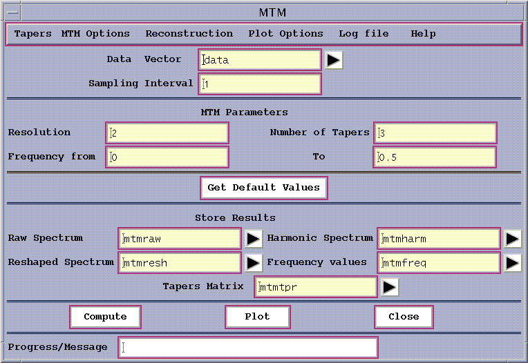
Figure 4: MTM window.
Having specified the data vector to be analyzed (here our 'data' vector with the SOI time series) and the sampling interval, there
are three MTM parameters that need to be specified. Again, a Get Default
Values button is provided as a guide, as well as a means to initialize
properly the `Frequency range' and a 'smoothing window width'
in MTM Options(see below) for the sampling interval not equal to one.
When changing the values of the sampling interval, the user has to ensure
correct scaling of the `Frequency range' and a
'smoothing window width' by changing them manually or by using
Get Default Values button.
Please note that the null hypothesis is effectively re-determined
whenever sub-interval of the
spectrum is analyzed. In this case an AR(1) spectrum is
fitted only to
that range, which will in general change the confidence levels,
and thus, potentially, the threshold for "reshaping" of the spectrum,
and detecting a harmonic peak!
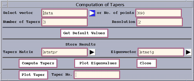
Figure 5: MTM Tapers window.
This allows one to compute and plot the tapers that are generated for
given choices of parameters.
There are several options in the MTM Options pull-down menu which
allow the user to change various settings from their defaults:

Figure 6: MTM options.
The choice of ``red noise''assumes a noise background that
consists of a temporally integrated Gaussian white noise or ``AR(1)'' noise
process. This null hypothesis is strongly motivated for dynamical reasons
in the study of geophysical phenomena, and represents the default option
of the Toolkit.
The choice of ``locally white noise'' assumes a colored noise
process that varies slowly but arbitrarily with frequency. This choice
is recommended if there is a priori reason to believe that the noise background
has a complex structure.
The choice of ``white noise'' represents a good null hypothesis
if absolutely nothing is known a priori about the physics or dynamics of
the process producing the noise background.
The choice ``narrowband'' will test the spectrum only for the
presence of narrowband signals, the former of the two possible signal detection
procedures described above.
The choice ``harmonic'' will test the spectrum only for the
presence of periodic signals, the latter of the two possible signal detection
procedures described above.
The choice ``N'' represents a convention in which the spectrum
is calculated per unit time by dividing by the length of the data series
in time units ``N'' (ie, a power spectral density). This is the default
convention, as it is throughout the Toolkit.
The choice ``none'' indicates a standard Fourier convention
of a finite length time series in which the spectrum scales with the number
of data points.
The user should be aware that chance statistics should lead to a 5%
rate of spurious harmonic signal detection at the 95% level, corresponding
to roughly 2-3 false positives over the Nyquist interval for a timeseries
of length N=100 time units, underscoring Thomson's (1982) general warning
that one should interpret with great caution significances of less than
about 1-1/N.
The ``raw'' option estimates noise parameters directly from the
unfiltered or ``raw'' time series. This option, albeit more traditional,
is generally discouraged. It should be selected, however, if the user is
interested in signals whose significance is measured only by the Thomson
variance ratio test for periodicity, without regard to their significance
as measured by their amplitude relative to the estimated noise background.
The median smoothing window width can be varied by the user within the
range 2 p f_Rayleigh to 0.25 f_N. In addition, the
``Misfit Criterion''
can be set to either a log fit or a linear fit
The ``linear fit'' employs a criterion which will weight the
robust fit of the noise background by the amplitude of the spectrum. This
choice is recommended if it is more important to fit the low-frequency,
high-power part of noise background.
Any results which show great sensitivity to the choice of ``log fit''
and ``linear fit'', or to the value of the median smoothing window f_smooth
over that range should be interpreted with some caution.
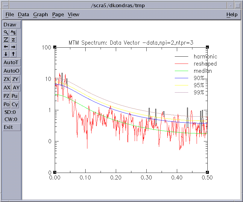
Figure 7: MTM Spectrum.
The MTM `Plot Options' pull-down menu on the main MTM panel controls launches the following window with default settings:
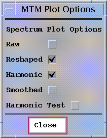
Figure 8: MTM Plot Options.
The choice ``raw spectrum''indicates that the raw MTM spectrum
should be displayed. Four additional smooth curves are shown, in increasing
vertical progression, for the median, 50%, 90%, 95%, and 99% significance
levels relative to the estimated noise background.
The choice ``reshaped'' indicates the estimated continuous
MTM spectrum or ``reshaped spectrum'' (the spectrum with estimated contributions
of harmonic signals removed). As above, signficance curves are also shown.
The choice ``harmonic spectrum'' indicates that the estimated harmonic or periodic component of the spectrum should be displayed. If the ``reshaped spectrum'' is also checked, the plot shows the estimated continous spectrum, along with a curve that rises above it to indicate the portion of the spectrum above the continuous background associated with a period signal. The latter component is shown as a narrow spike of breadth equal to the spectral estimation bandwidth.
The choice ``smoothed'' will plot the median-smoothed spectrum, if it
was computed.
The choice ``harmonic peak test'' indicates that the variance-ratio
test for significance of harmonic signal detection should be shown as a
function of frequency. Also shown are the median, 90,95,and 99% confidence
levels for significant detection of a periodic signal relative to the assumption
of locally-white noise.
As we can see from the Fig.7 and Components Frequency Selection list
of MTM Reconstruction window in
Fig.9 (see below), the MTM analysis identifies
two highly significant peaks, one centered at f=0.0146, and another
centered at f=0.0342. The signals are significant at well above the
99% level. We associate thease peaks with the low-frequency LF(band)
and high frequency (HF) band ENSO signals. A weak trend is also
identified at f=0.001.
The black peaks indicate harmonic signals selected in the Reshaping procedure.
There are 8 such peaks including both an
LF and HF ENSO band peak.
Selecting the `Reconstruction' pull-down menu on the main MTM panel
allows the user to perform time reconstructions of any of the signals identified
as signficant in the spectrum analysis, via the following window:

Figure 9: MTM Reconstruction window
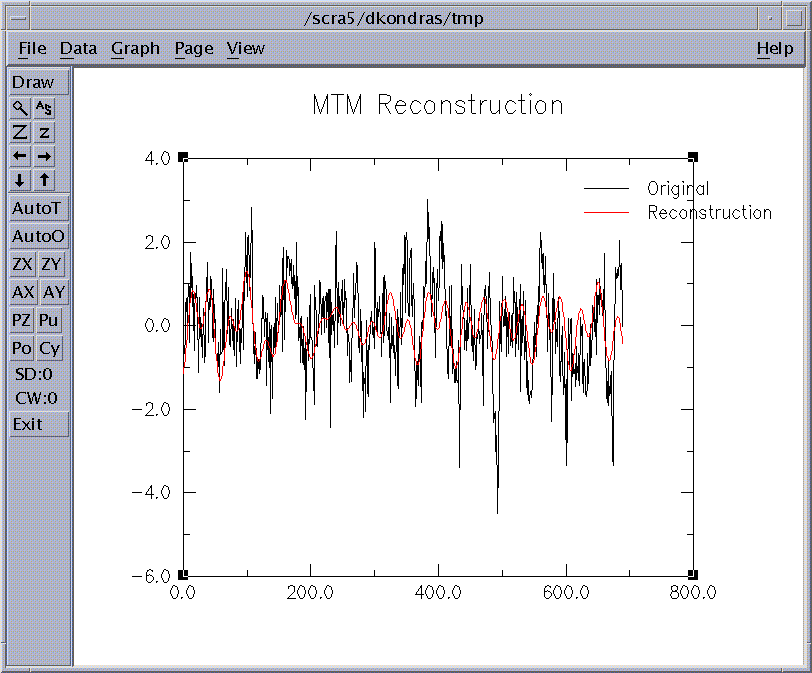
Figure 10: MTM Reconstructed signal.
 |
 |
 |
 |