3. TOOLKIT DEMONSTRATION
e. Singular-Spectrum Analysis
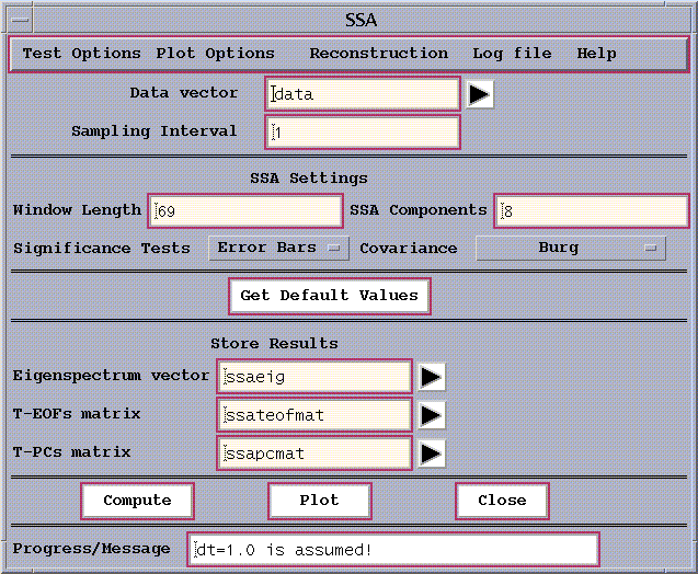
Selecting the `Singular Spectrum Analysis' button from the Analysis
Tools menu on the main panel launches the following window
(shows its state after pressing Get Default Values button, see
below):

Figure 11: SSA control panel.
Having specified the data vector to be analyzed (here `data', the SOI time-series) and the sampling interval, the principal
SSA options to be specified are the Window Length, the type of Significance
Test, and Covariance Estimator. The number of SSA Components
specifies how many components will be retained for future analyses. The
Get Default Values button is provided as a guide.
Window Length
As a rule of thumb, the window length M should be chosen to
be longer than number of data points in the oscillatory periods under
investigation, and shorter
than number of data points in the spells of an intermittent oscillation. Vautard et al. (1992) recommend
that the window length be less than about N/5 where N is the number of
points in the timeseries. Robustness of results to M is an important test
of their validity. The choice of window length sets the dimension of the
lag autocorrelation matrix to be constructed and diagonalized by SSA, and
thus determines the computational burden of the application. Larger values
of M correspond to higher spectral resolution, although there is no direct
equivalence between them.
We will set the Window Length to 60, which is a good choice
for out time series (690 data points with a one month sampling rate) and the oscillatory periods
(2 and 4 years) under investigation.
Covariance Estimation
The method for estimating the autocovariance matrix that is decomposed
(diagonalized) by SSA is chosen by selecting either `Burg' , `Vautard
-Ghil' , or ` Broomhead &King ' from the `Covariance'
button on the main SSA control panel (Fig. 11).
As indicated in the theoretical section, Burg estimation is an iterative
process based on fitting an AR model with a number of AR components equal
to the SSA window length. The Burg approach in principal should involve
less "power leakage" due to the finite length of the time series and should
therefore improve resolution (Penland et al., 1991). However, Vautard et
al. (1992) found that the Burg estimate can induce significant biases when
nonstationarities and very low-frequency variations are present in the
series. Thus in some cases it will be worthwhile to try the Vautard et
al. method. Also, for long series (N on the order of 5,000), the Vautard
-Ghil estimate is less computationally burdensome and thus is completed
more quickly.
In practice, we have found that the Vautard-Ghil method is more prone
than is the Burg method to numerical instabilities (yielding negative eigenvalues)
when pure oscillations are analyzed. Both the Burg and Vautard-Ghil methods
impose a Toeplitz structure upon the autocovariance matrix whereas the
Broomhead & King method does not. The Broomhead & King method is
thus somewhat less prone to problems with nonstationary time series (Allen
et al., 1992b), although the Vautard et al. method seems untroubled by
all but the most extreme nonstationarities. The Toeplitz methods also impose
symmetries on the EOF shapes whereas the Broomhead & King method does
not. However the Toeplitz methods do appear to yield more stable results
under the influence of minor perturbations of the time series (Allen and
Smith,1996).
NB: The Burg covariance matrix estimation option is not supported by
MCSSA which defaults to Vautard-Ghil if Burg is selected on the main SSA
panel.
We used Burg covariance method for analyzing SOI time series.
Significance tests
There are three choices for Significance test
-
Error Bars
-
Chi-Squared
-
Monte Carlo SSA
described below. If Error Bars are selected, the eigenspectrum is
displayed in order of eigenvalue rank. In the remaining two cases, the
spectrum of eigenvalues is plotted against the dominant frequency associated
with the respective T-EOF.
Exception: the eigenspectrum-shape
test in MCSSA is plotted against rank.
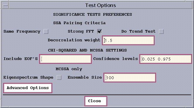
The Test Options
pull-down menu is used to set the preferences for the particular test, and is shown in Fig. 12. These options are explained in more details below.

Figure 12: Test options control panel.
Error Bars Test
This is the default test. It constructs a set of ad-hoc error bars that are
based on the estimated decorrelation time of the time series according
to:
dli = (2kL/N)1/2 li
where L is a typical decorrelation time for the time series, k is
a user supplied Decorrelation weight between 1 and 2 (1.5 by default), and li is the i-th eigenvalue in the spectrum. The Toolkit estimates
L to be the inverse of the logarithm of the lag-one autocorrelation of
the time series. Weights close to 1 are closer--but not generally equal
to--the liberal error bars of Vautard and Ghil (1989); weights approaching
2 are closer to the conservative error bars of Ghil and Mo (1991a).
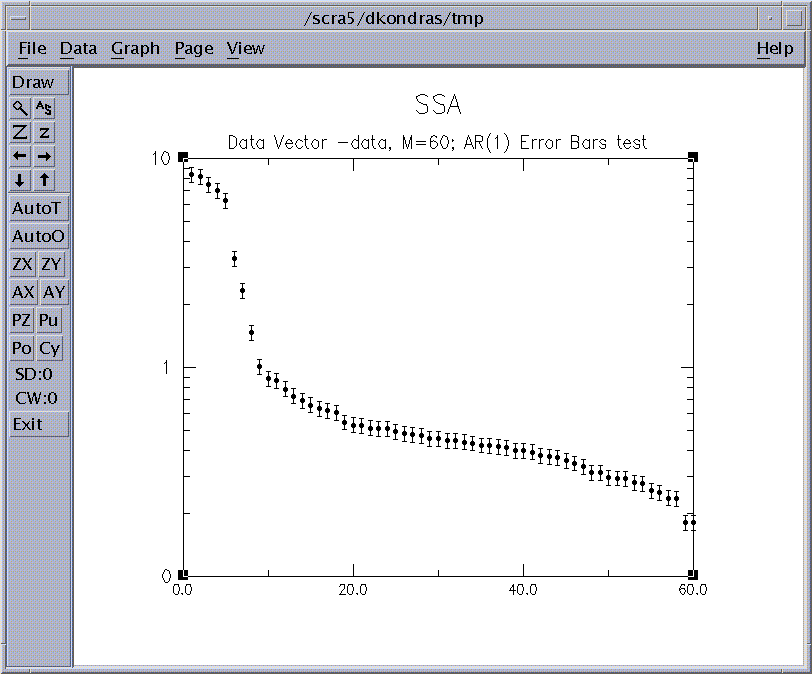
After we click the Compute
and Plot buttons a graphics window will open to display the eigenvalue
spectrum of the specified SSA.
The units of abscissa are SSA component number (eigenvalue rank), and with
the variance contributed by each SSA component on the ordinate.

Figure 13: SSA eigenvalue spectrum for 'soi'.
Since the window length was set to 60, SSA decomposes the time series into 60
components and thus 60 eigenvalues are plotted. The significance of the various
components can be judged qualitatively by noting which components contribute significantly
more variance relative to the noise background. The latter in turn
assumed to include the components that lie in the flattish tail of the eigenvalue spectrum, i.e.
components from about 10 to 60.
The leading 10 components in figure 11 lie above a distinct break in the eigenvalue
spectrum, and thus may be of physical significance. In particular, we
are interested in the leading four components which form two pairs of nearly equal eigenvalues.
As discussed in the theory section above, pair of nearly equal eigenvalues
in SSA is one of the characterising as oscillation.
However, the eigenvalues are subject to
numerical and sampling errors (North et al., 1982), and mere pairing of eigenvalues is not enough
to guarantee that an oscillation has been identified. In the eigenvalue plot above, the error bars show an
ad hoc range of the estimation errors. (See below for more
sophisticated significance tests.) Any of the eigenvalues with significantly overlapping error bars
could represent an "oscillatory pair'. Also eigenvalues with error bars that overlap significantly
with the error bars of the noise part of the spectrum must also be suspected of being part of that
noise.
Pairing Criteria
The Toolkit identifies potential oscillation components
using 3 pairing criteria which can be activated concurrently
using checkboxes in Fig. 12. (These 3 tests are performed on clusters of
eigenvalues whose ad-hoc error bars overlap; however, it is not necessary
for the 'Error Bars' test to be selected on the main SSA panel.) The results
of these tests are written to the log file.
In the SOI example, the log file shows that component 1-2 meet both criteria for
being oscillations. We will return to investigate the oscillations after considering some more of the
controls in the SSA part of the menu.
Monte Carlo SSA and Chi-Squared test
The Monte Carlo SSA (MCSSA) significance test is described by Allen and
Smith (1996). It tests significance against a red noise null-hypothesis.
You may download
test dataset of Allen and Smith (1996), if you want to reproduce the figures in that paper.
A large ensemble of red-noise surrogate time series are generated, each
with the same length and same expected lag-1 autocorrelation as the time
series to be tested (but see note under 'Include EOFs' below).
Two fixed T-EOF bases are used, unless the eigenspectrum-shape test
is invoked (see below).
-
The data, together with many AR(1) noise realizations are projected onto
the EOFs of the data covariance matrix, i.e. the "data basis".
-
The data, together with many AR(1) noise realizations are projected onto
the EOFs of the expected covariance matrix of pure noise, plus any selected
"signal" EOFs of the data covariance matrix which are specified as "included"
(see below) in the null-hypothesis, with the rest as for pure noise, after
orthogonalizing. See Allen and Smith (1996) section 4.4. This is called
the "null-hypothesis basis", and it is either pure noise, or a "hybrid
basis" of noise plus certain data EOFs. The noise covariance matrix is
computed analytically from the estimated lag-1 autocorrelation coefficient
of the test time series.
If certain data EOFs are "included", the resulting "hybrid basis"
is the most reliable if you have already identified a strong signal in
your data (e.g. an annual cycle), which would otherwise overwhelm the noise
parameter estimation.
`Include EOFs box': List of "signal" EOFs (by rank) to include in
the noise null-hypothesis, from which the noise surrogates and null-hypothesis
EOFs are computed. Note that irrespective of basis (data or null-hyp. EOFs),
the characteristics of the noise, and thus the error bars are modified
by including data EOFs. In fact the contribution of the latter to the lag-1
autocorrelation of the data time series are removed, when they are included
in the null-hypothesis, see Allen and Smith (1996). If no data EOFs are
specified, the null-hypothesis is pure AR(1) noise. Set of space-delimited
integers. Not relevant to the 'Monte Carlo Eigenspectrum shape' test.
`Confidence levels box': Pair of confidence levels of the noise
null-hypothesis to plot. For example, 0.05 and 0.95 would plot noise error
bars spanning the 5th to 95th percentiles of the noise distribution. Two
space-delimited reals.
`Ensemble Size': Number of Monte Carlo noise realizations.
Eigenspectrum Shape Monte Carlo test
`Eigenspectrum shape checkbox': This checkbox makes a fundamental
change to the nature of the Monte Carlo test, making it a separate test.
This test based on eigenspectrum shape, in which a new EOF basis is computed
for each noise realization by diagonalizing its individual covariance matrix--
see Elsner and Tsonis (1994) or Dettinger et al. (1995). The ranked eigenvalue
spectrum of the data is plotted along with chosen percentiles of the ranked
eigenvalue spectra of the noise realizations.
Advanced Options: This button yields a control panel that allows
the MCSSA "Data Basis", "Noise Basis" and the set of surrogates to be saved
to a file, or read (NB: read function not yet implemented - sorry!)
in from one. This may be useful if you want to use a custom-made basis,
or you want to save a large ensemble of surrogates for future use. The
red-noise coefficients used to generate the surrogates can also be overidden
by inputting values here. Warning: If these files are not in the correct
format, the Toolkit will crash!
Note on MCSSA temporary files: The MCSSA and Chi-squared tests
generate a set of local files mcssac.* that are deleted upon exiting the
Toolkit. If these files are needed, they must be copied/moved by hand using
Unix.
Chi-squared test
It follows the Monte Carlo SSA (MCSSA) approach
(see above) in which red-noise surrogates are projected onto the basis
consisting of the SSA eigenvectors (T-EOFs) of either the data or null-hypothesis
covariance matrix. In contrast to MCSSA, the chi-squared test approximates
the distribution of surrogate projections as chi-squared with 3M/N degrees
of freedom. This is quite accurate for the case of sinusoidal EOFs and
a linear (AR-type) noise null-hypothesis -- see Allen and Smith (1996),
appendix. The probability of n excursions above the mth percentile is then
estimated using the binomial distribution. This method is computationally
fast compared to MCSSA which generates a large ensemble of surrogate noise
series.
A typical testing procedure for Monte Carlo or Chi-Squared tests would be as follows (i)
begin by testing against pure noise and identify frequencies at which the
data displays anomalously high power against this null-hypothesis; (ii)
find the data EOFs which correspond to these frequencies (being data-adaptive,
these will often provide a better filter for the signal than the corresponding
EOFs of the noise); finally (iii) re-test including these EOFs in the null-hypothesis
to check if there are other features in the spectrum which were concealed
by the dominant signal . It is, of course, consistent to iterate this procedure,
but beware of the problem of test multiplicity discussed in Allen and Smith
(1996) section 4.2: iteration makes the test increasingly liberal, so results
which are still on the margins of acceptable significance after a couple
of iterations including successively more EOFs into the "signal" should
be ignored.
Accordingly, to test against a pure red-noise null-hypothesis,
we choose Chi-Squared as a significance test in the
Test Options panel, leaving the Include EOFS field blank,
as in Fig.12.
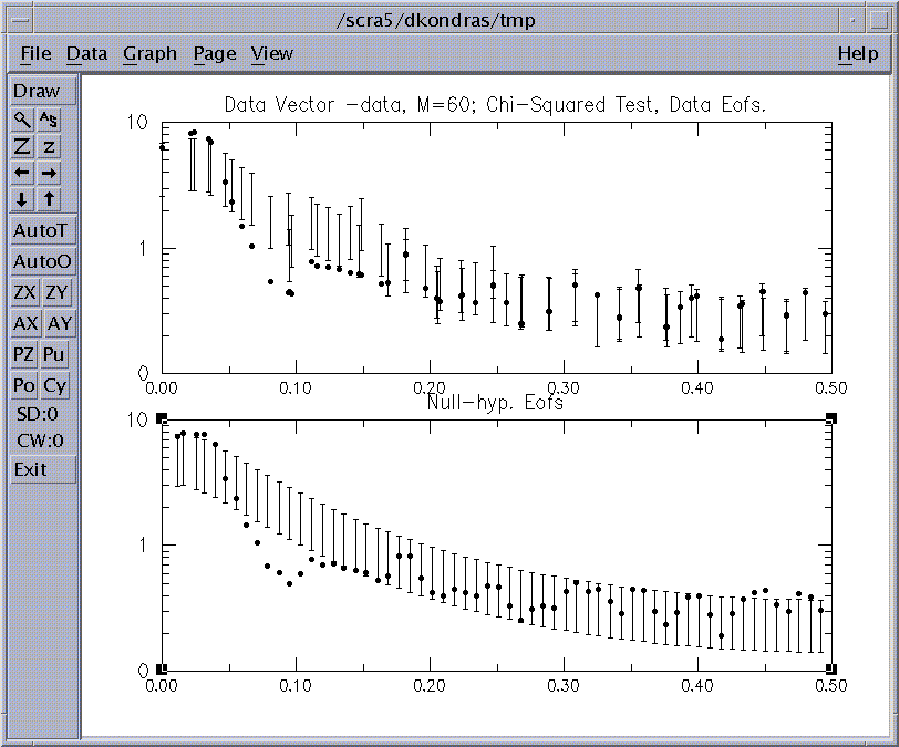
After clicking the Compute and Plot buttons,
the following graphics window will open:

Figure 14: Chi-Squared test for 'soi'.
Both parts of Fig.14 have variance plotted against the dominant
frequencies of 'basis'
EOFs on x-axis, and describe projection of data and null-hypothesis (NH) surrogates onto 'basis' EOFs (see above). The dominant frequencies of EOFs are calculated with a 0.001/dt resolution in the Nyquist interval from 0 to 0.5/dt. The error bars represent 95% of variance
(with settings of Confidence levels such as in Fig. 12) we expect to find
in the state-space direction defined by a particular EOF from the 'basis',
when analysing a segment of 'NH' noise. Using 'Include EOFS' option we can
construct a composite 'NH' as described above, but it is a pure red-noise here.
For the upper graph the 'basis' consists of the EOFs of the 'data' covariance matrix, and the projection of data gives us SSA
eigenvalues plotted as dots.
For the lower graph, 'basis' EOFs are computed from the expected covariance
matrix of the 'NH'. Projection of data does not give SSA eigenvalues here,
but the interpretation of the graph is the same.
Note how the EOFs of the pure noise NH are almost regularly spaced. According to
Allen and Smith ('96) the NH basis avoids artificial varaiance-compression
inherited in SSA and therefore it has a lower probability of
false-positive results, i.e. identifying the noise components as significant.
For the Data Eofs basis
we observe that eigenvalues corresponding to EOFS 1-2
and 3-4
appear almost superimposed on each other at frequencies equal to ~ 0.02 and 0.034 cycle/month, and lie outside the null-hypothesis error bars.
Thus they are relatively unlikely ( at the 95% level, with settings of Confidence levels such as in Fig. 12.) to be merely due to selected
null-hypothesis process, and represent two signficant oscilattions.
The NH basis (lower graph) confirms the significance of these pairs, and we
conclude that they correspond to the QB and QQ components of El Niño.
The results of the Chi-squared test should always be checked using the Monte Carlo approach,
which is also essential with more complex noise models. We leave it as an exersise to the reader to check that similar results are obtained for our SOI time series with the Monte Carlo SSA test.
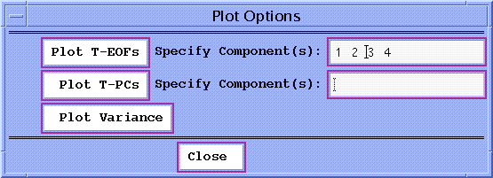
The T-EOFs, T-PCs and variances can be plotted using the Plot Options
pull-down menu:

Figure 15: SSA Plot Options.
-
`Plot T-EOFs' --Clicking this button creates a plot of the temporal
EOFs typed into the Specified Components box alongside (space delimited
integers).
-
`Plot T-PCs' --Clicking this button creates a plot of the temporal
PCs specified.
-
`Plot Variance' --Clicking this button creates a plot of normalized
eigenvalues. The units of the ordinate are percent of the total timeseries
variance.
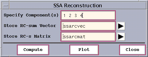
The Reconstruction pull-down menu on the main SSA panel allows the
reconstruction of the original timeseries from selected SSA components,
specified as a space-delimited set of integers:

Figure 16: SSA Reconstruction Window.
Selecting the identified 'significant' components 1-4, and
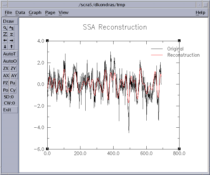
After hitting the Compute and Plot buttons,
a following graphics window will open:

Figure 17: SSA Reconstruction.
Here the reconstructed signal is plotted against original timeseries, with a mean average removed.
If this SSA-filtered RC series ('ssarcvec' vector) is now analyzed by MEM or MTM, the frequency spectrum of the RCs
is much simpler than that of the complete time series, since most of the "noise" has been removed
(Penland et al. 1991, Keppenne and Ghil 1992).
The MEM Spectrum of SOI RCs series is plotted in Fig. 3c.
We leave as an excersise for the user to repeat SSA analysis with 11
SSA Components, and try to identify pair 10-11 with the oscillatory signal. Hint: this is related to the peak in
MTM Spectrum at f~0.18 cycles/month.
Last modified: September 6, 2000


