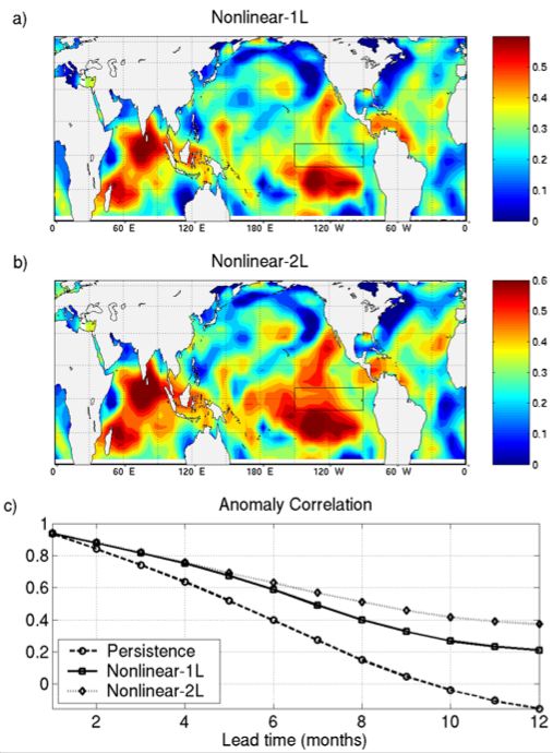
The 1-L and 2-L nonlinear (quadratic) models are compared in terms of their respective forecast skills in Fig.4. Spatial distribution of SST anomaly correlation of 9-month lead forecast for the 1-L and 2-L models is shown in panels (a) and (b), respectively. The forecast time series is a 100 member ensemble mean of models' stochastic realizations, and it has been cross-validated over the whole time series as described above.
Although both models have similar skill patterns, the 2-L model's forecast skill is higher than that of its one-level counterpart, especially south of the Nino-3 region,
shown as the black box in panels (a) and (b).
The correlation between the observed and predicted area-averaged Nino-3 SST anomalies is plotted in panel (c): the 2-L model is getting significantly better than a 1-L model at lead times longer than 4 months; both 1-L and 2-L models beat persistence forecast.
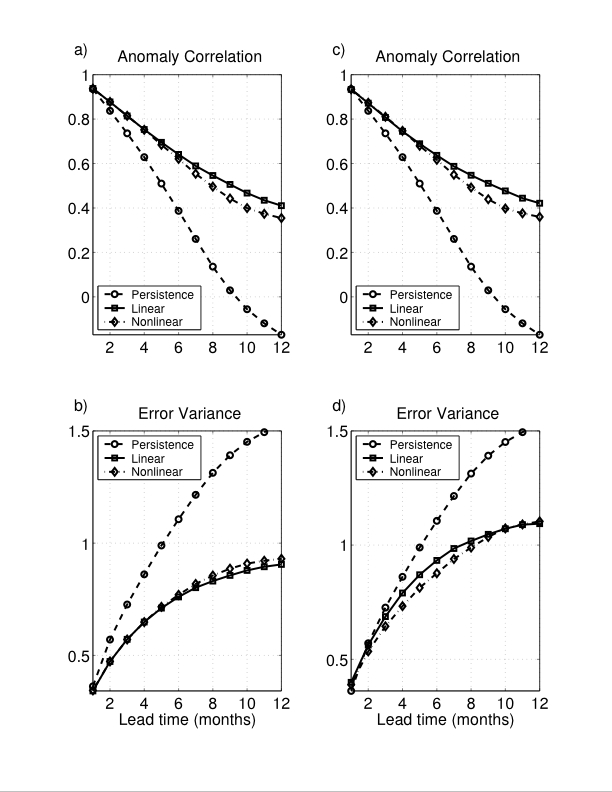
Next we compare 2-L linear and nonlinear models. The anomaly correlation coefficient and normalized prediction error varaince, are shown in Fig.5 for the cross-validated Nino3 SST forecasts: (a) and (b) for the 100-member ensemble mean, (c) and (d) for the extreme event forecast series, which are defined as the weighted sum of the top and bottom 20% of ensemble forecast. Such a time series produced by a quadratic model has a smaller rms error than that of its linear counterpart [panel (d)], with both models' anomaly correlation being essentially the same as for the ensemble mean forecast [compare panels (c) and (a)]. This improvement of the quadratic versus linear forecasts comes from the ability of nonlinear model to capture non-Gaussian PDF distribution characteristic of ENSO, with positive anomalies having larger amplitude than the negative anomalies, while the PDF distribution of the linear inverse model time series is normal. The linear model tends, therefore, to underestimate the magnitude of El Nino events, and, likewise, to overestimate that of La Nina events.
Figure 4. Comparison of the one-level (1L) and two-level (2L) nonlinear models' performance. Anomaly correlation at month 9 (9-month-lead forecast) with cross-validation: (a)1-L model; (b) 2-L model; (c) Nino-3 SST anomaly forecast skill as a function of a lead time for 1-L model, 2-L model, and persistence forecast, lines are defined in the legend. Nino-3 SST anomaly is defined as the area-average over the box shown in panels (a) and (b).