

 |
 |
 |
 |
Type `Spectra', hit <return> and the main Spectra window will appear:

Figure 1a: Main `Spectra' window.
There are five pull-down menus, plus a `Help' button for a brief description of each.
The `Exit' button quits all tools, and any results are lost unless they have been explicitly saved. Any open plot windows remain, however. The toolkit creates a number of local files while running. These files will be ALL DELETED !!! after exiting the program.
Before applying any of the Toolkit tools, the file containing the time series to be analyzed must be read in.
Data should be in the form of ascii columns, and can be either a column vector of a single time series, or a matrix of several columns, one for each time series. The 'Read Vector' or 'Read Matrix' functions from the File/Data menu are used to read the data. However, if a multi-column file (matrix ) is read using 'Read Vector', only the second column is read into a vector, while the first column, assumed to be time values, is ignored.
Values in the time series must be equally spaced in time. The sampling interval is assumed to be unity by default. If it is not unity, each tool needs to be told individually what the sampling interval is using the "Sampling Interval" box (see below). The resulting spectra are then plotted accordingly. If, for example, the data are sampled every 2 months instead of monthly, the Nyquist interval on the frequency axis will be labled from 0 to 0.25 cycles/month.Throughout the Toolkit the spectrum is calculated per unit time by dividing by the length of the data series in time units ``N'' (ie, a power spectral density). This is the default convention.
We will work through examples using each tool on a time series of monthly values of the Southern Oscillation Index (SOI), a climatic index that chracterizes El Niño (Bjerknes, 1969). The 690 month series `soi' was obtained from monthly mean sea-level pressures at Tahiti and Darwin, Australia, by removing their seasonal cycles, dividing the resulting anomalies by the corresponding standard deviations, and then taking the Tahiti-minus-Darwin difference. The SOI series considered here is for the time interval from January 1942 through June 1999, during which no observations are missing.
It is also included in a source code dsitribution. To read the SOI time series, we use the 'Read Vector' function, which opens the following window:
Figure 1b. `Read Vector' window.
This window allows you to browse a list of files, select a file and then read it and store in a named vector. SSA-MTM Toolkit allows you to handle many time series at once; these might typically be a raw input time series and a filtered series derived using the Toolkit. These time series and results of the computation are stored internally as vectors or matrices, each of which needs to be given a name.
To choose the time series `soi' for analysis, either:
The user has access to vectors and matrices via window lists, which show the names and dimensions (Fig. 1c.), i.e. the number of elements in a vector and number of rows and columns for a matrix. List windows are activated by pressing on the arrow buttons located next to the boxes with the name of the vector or matrix, see Fig. 1.b.
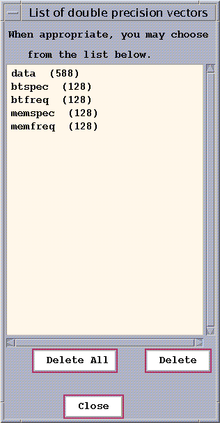 | 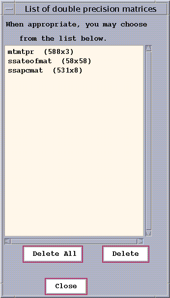 |
Figure 1c: 'Vector List' and 'Matrix List' windows.
To make a plot of the time-series data, we go to the 'Vector' function in a pull-down Plot menu, which opens the following window:
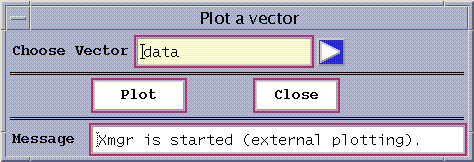
Figure 1d: 'Plot Vector' window.
This window allows the vector elements to be plotted against their index. The user has to specify the name of the vector from the vector list. By pressing on the 'Plot' button, a new graphics window opens with a plot of SOI time series:
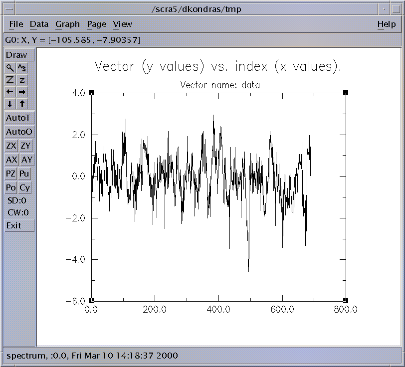
Figure 1e: SOI Time series.
The time series `soi' that we have read in is noisy, with no obvious oscillatory components. Our goal is to identify the low-frequency quasi-quadrennial (QQ) and quasi-biennial (QB) components of El Niño (Rasmusson et al., 1990).
When selecting Options in the pull-down menu for Plot on the main panel, the following window will open:

Figure 1f: Graphics options

Figure 1g: SOI plot by IDL.
IDL plots are created with the script files written out
by the Toolkit whenever the Plot button is pressed for any of the plotting
functions. The name of the script file is given by the
variable 'BATCHFILE', (see Fig. 1i below) i.e. 'vector.idl.tmp' for our
example.
In IDLDE window the user can perform further analysis
by starting IDL Insight, or by running their own
IDL scripts using the plot data imported into IDLDE (as seen below in Fig. 1i).
We can create a postscript file idl.ps of the plot in Fig.1g by entering at IDL propmt SET_PLOT, 'PS', and then
@vector.idl.tmp.
Please note that IDLDE and Insight are features of the IDL version 5.0 and later.
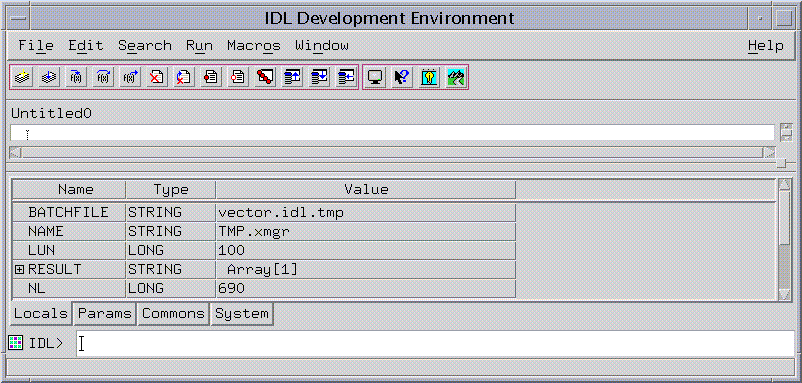
Figure 1i: IDLDE window.
 |
 |
 |
 |