Table of Contents
Introduction
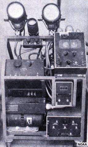
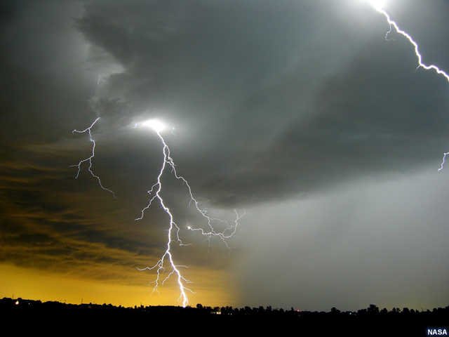
Radar technology has been used since World War II when military personnel tracking enemy aircraft and ships discovered that precipitation also appeared on radar displays. By the end of the war radar technology had advanced considerably, and scientists began using surplus radars to study and monitor weather features.
Today, weather radars are usually one of the main tools in the forecaster's arsenal.
This 2-hour module discusses the fundamental principles of Doppler weather radar operation and how to interpret common weather phenomena using radar imagery. Although intended as an accelerated introduction to understanding and using basic Doppler weather radar products, the module is also an excellent refresher for more experienced users.
By the end of this module, users will be able to:
- Explain the basic principles of weather radar operation
- Describe the primary uses and limitations of radar data as well as factors that affect data quality and interpretation
- Interpret wind speed and direction using Doppler radial velocity imagery
- Interpret precipitation intensity and movement using radar reflectivity imagery
- Use radar imagery to identify phenomena that commonly occur during otherwise fair weather including dust storms, smoke, horizontal convective rolls, fronts, and other boundaries
- Use radar imagery to identify common features of precipitating phenomena, such as winter storms, convection, and tropical cyclones
- Use radar imagery to identify instances of anomalous propagation, velocity and range folding, non-meteorological targets, and other radar artifacts
Overview of Weather Radars
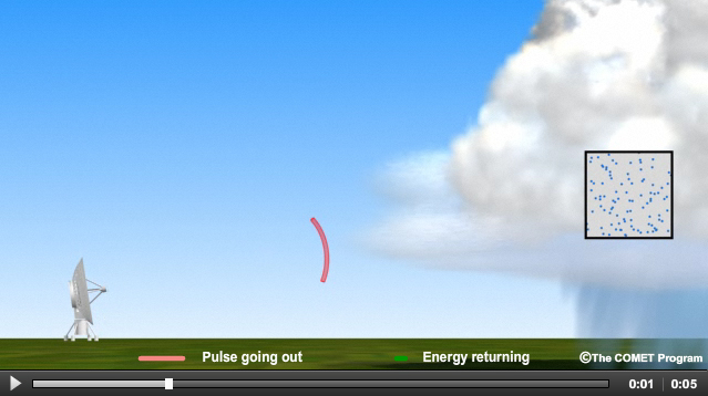
A weather radar works by emitting pulses of electromagnetic energy at microwave frequencies into the atmosphere. When these pulses encounter objects , some of the electromagnetic energy is scattered back toward the radar. This is often referred to as being "reflected" back, and is where the term "reflectivity" comes from. Reflectivity is a measure of a radar target's efficiency in intercepting and returning the radar's energy and depends on the physical parameters of the targetits size, shape, orientation, composition, etc.
The energy received back to the radar is analyzed by computers to determine the location and intensity of precipitation, and information about the wind speed and direction. The information is then plotted on images.
In order to make the best use of radar products, it is important to understand fundamental operating principles of common weather radars, which are covered in this chapter. This information will enable a forecaster to forecast short-term precipitation trends, general wind patterns, and hazardous conditions. Additionally, forecasters will be able to recognize false radar echoes and other problems with radar images, which are discussed in the next chapter.
Types of Weather Radars
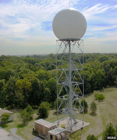
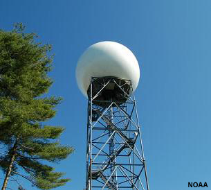
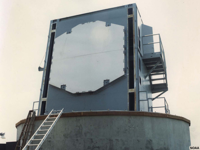
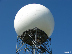
A National Weather Service NEXRAD tower and radome, which houses the antenna
Many types of radars are used to detect precipitation and other weather conditions. The most common ones used in the United States are those pulse radars that make up the National Weather Service's NEXRAD (NEXt Generation RADar) WSR-88D system and the less common, but more sophisticated, phased-array radars used mainly by the military and in atmospheric science research.
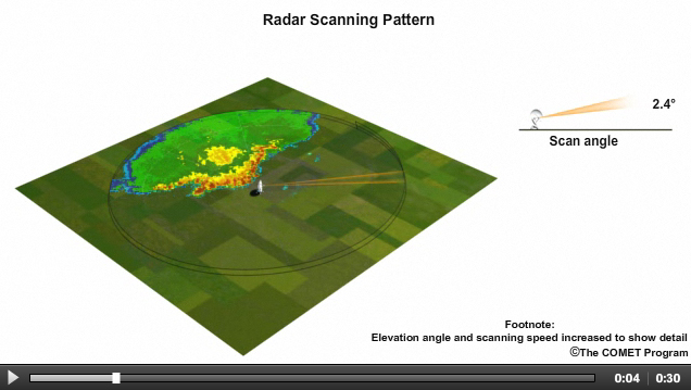
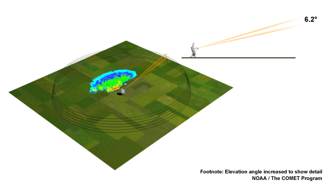
Typically, a NEXRAD WSR-88D radar antenna is pointed at a low angle, sends out a pulse for a fraction of a second, and then "listens" to receive any returning energy or "scattering." Then the radar rotates an incremental amount and repeats the process. Once the radar completes an entire revolution, the antenna elevation angle is increased and the process is repeated. Radars transmit and listen so quickly that they can scan much of the nearby atmosphere in about 5 minutes.
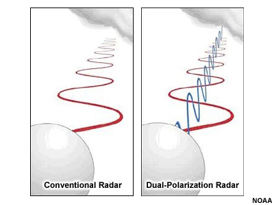
The National Weather Service is currently upgrading their pulsed radar network to dual-polarization radars. WSR-88D radars emit and receive pulses that have horizontal orientations. Dual-polarization radars also transmit and receive data in the vertical direction, providing a more complete picture of atmospheric targets.
This technology allows forecasters to:
- Identify non-weather targets more easily
- Differentiate rain, snow, and melting snow
- Detect when hail is present in a thunderstorm
- Detect debris lofted by strong tornadoes
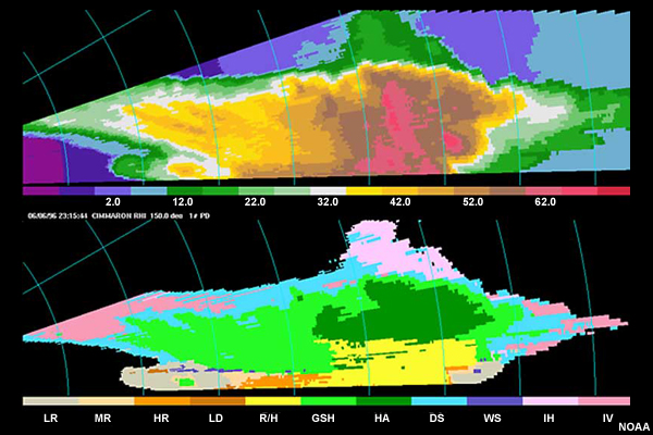
Vertical cross-section view of dual-polarization reflectivity (top) and precipitation type (bottom). The bottom color scale progresses from light-moderate-heavy rain through rain/hail mix, graupel/sleet, hail, dry and wet snow, and ice.
Deployment of the systems began in 2011, and completion is expected in 2013. The new radar products, some of which may have limited availability to outside users, will have significant changes that are not discussed in this module. More information is available from the NWS Warning Decision Training Branch.
By contrast, phased-array radars do not have a single rotating antenna and instead direct electromagnetic pulses via arrays of many small antennas. Most have dual-polarization capabilities as well. This type of radar will likely replace the WSR-88D radars in the future.
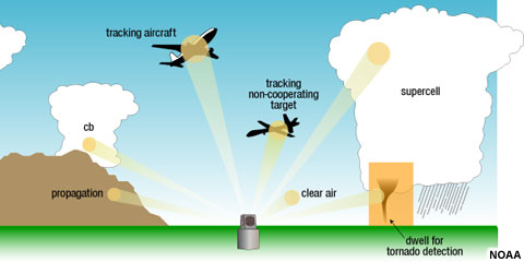
Illustration of phased array scans including a scan through a cumulonimbus (cb) cloud; detection and tracking of aircraft; scan through the planetary boundary layer (clear air) for mapping winds; scan through a supercell storm; and long-dwell scan through a region of a potential tornado
Because no mechanical rotation or inclination is involved, phased-array radars can scan much faster and in any specific area that is desired, such as an individual thunderstorm cell. They can also be used to scan multiple areas of interest simultaneously.
For most applications, the phased radar returns look quite similar to those of NEXRAD WSR-88D pulse radars and interpretation of them is very similar.
Scanning Modes
There are two common scanning modes for a NEXRAD WSR-88D radar: precipitation and clear air.
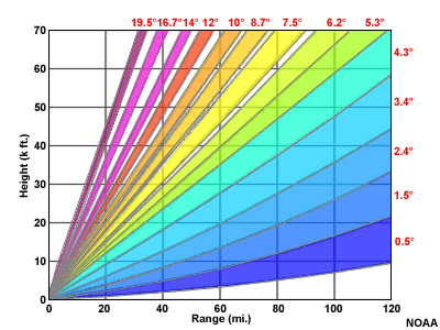
Precipitation Scan Mode: NEXRAD WSR-88D radar beam heights with distance for different antenna elevation angles (red numbers) used in a precipitation volume scan pattern
Precipitation mode is used when precipitation is occurring or is expected in the forecast area. In this mode, the radar scans several elevation levels using a pulse repetition frequency (PRF) that allows forecasters to quickly receive information about the atmosphere.
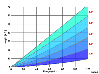
Clear Air Scan Mode: NEXRAD WSR-88D radar beam heights with distance for different antenna elevation angles (red numbers) used in a clear air mode volume scan pattern
Clear air mode is used when no significant precipitation echoes are in the area, to examine very light precipitation or other particulates, and to detect subtle boundaries or fronts. Lower elevation angles are used since this is primarily where clear air targets such as dust, birds, and insects will be located.
Notice that there is a significant portion of the troposphere directly above the radar that is not scanned. This area is referred to as the "cone of silence."
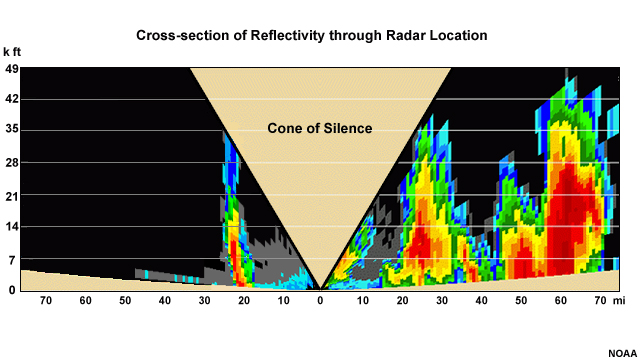
This is not usually a problem when precipitation is widespread and light-to-moderate, but it can mean that the top portions of thunderstorms within about 20 km (12 miles) will not be observable.
Reflectivity
NEXRAD WSR-88D radars are designed to detect scattering from specifically-sized targets within approximately 200 km (124 mi) of the radar. The amount of energy received back by the radar (about 1 nanowatt) is typically much, much smaller than the initially transmitted pulse (usually 1 megawatt). The radar receiver amplifies this returned scatter and uses its amplitude to calculate the "radar reflectivity factor" (Z).
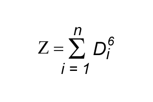
The radar reflectivity factor is proportional to the sum of the sixth power of the diameter (D) of all of the scattering targets in the sample volume. Since raindrop size is usually measured in units of millimeters, and volume is usually expressed in units of cubic meters, the radar reflectivity factor has units of mm6/m3.
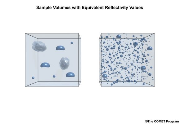
This sixth power dependence means that large particles dominate the calculated reflectivity value. In this example, we see that just a handful of large raindrops and small hailstones produce the same reflectivity as hundreds of small raindrops.
Reflectivity Scales
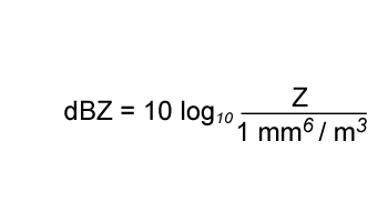
Typical values of radar reflectivity factors for non-precipitating clouds or light drizzle would range from 10-5 to 10; for very heavy rain and hail the factor would be as high as 107. Because these values range over several orders of magnitude and are difficult to depict graphically in much detail, radar products typically use an easier-to-interpret logarithmic scale of dBZ (decibels of Z).
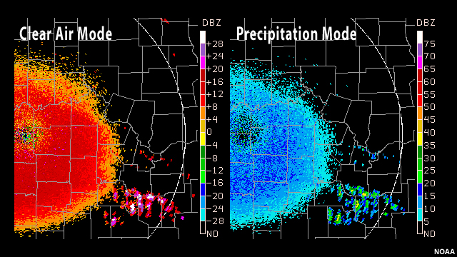
The scales usually span from -28 to +28 for clear air mode and 0 to 75 for precipitation mode.
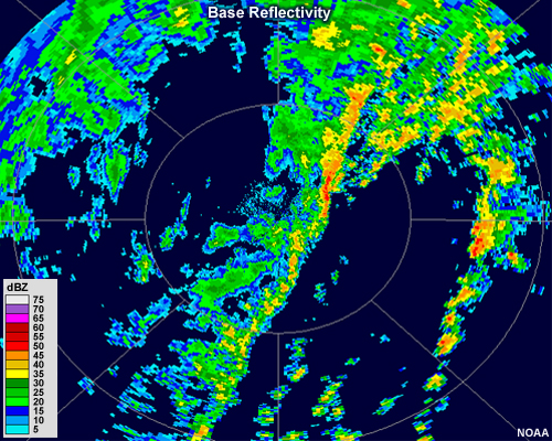
In precipitation mode, low dBZ values (blue and green colors) indicate light precipitation, while higher values in the yellow, orange, and red colors mean heavier precipitation. Values above about 45 dBZ signify intense precipitation and are nearly always caused by thunderstorms. Anything above 60 dBZ generally means that the sample volume contains some hail.
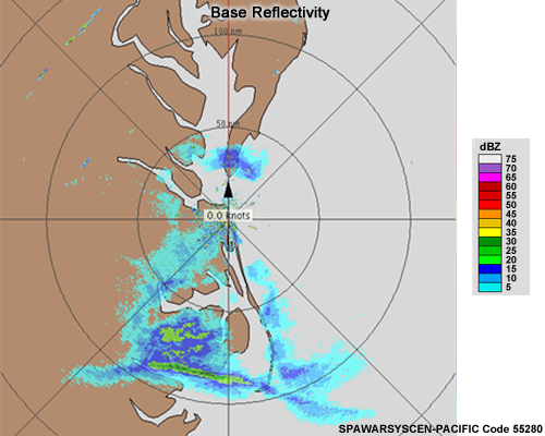
Reflectivity Products
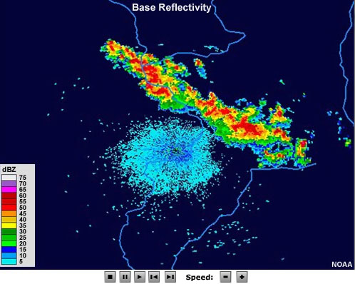
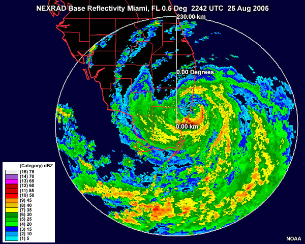
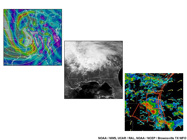
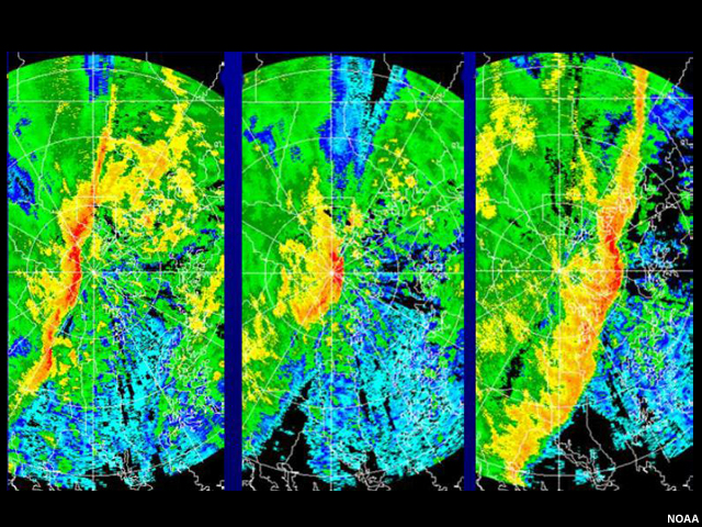
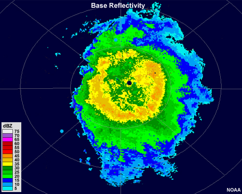
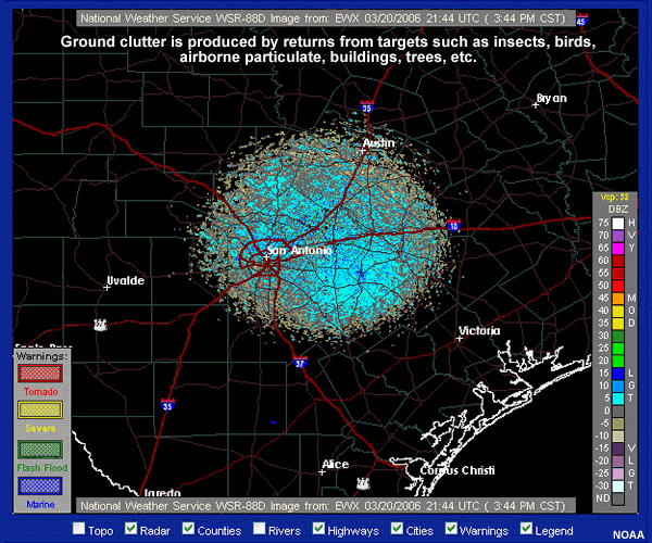
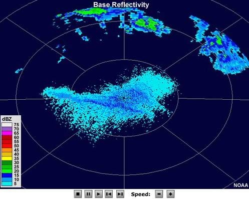
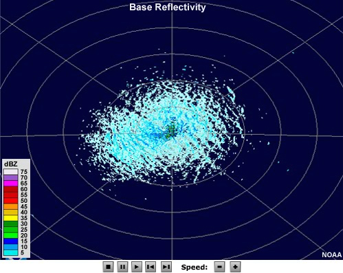
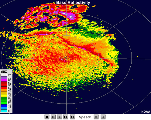
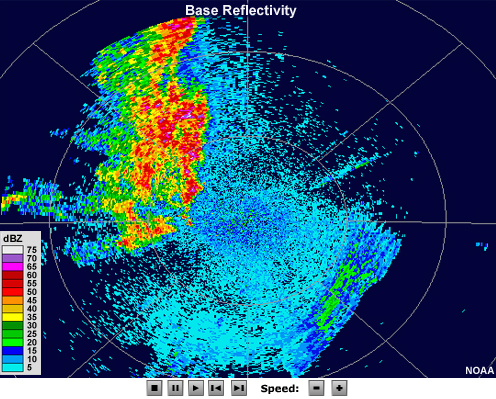
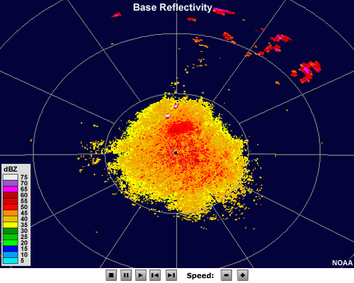
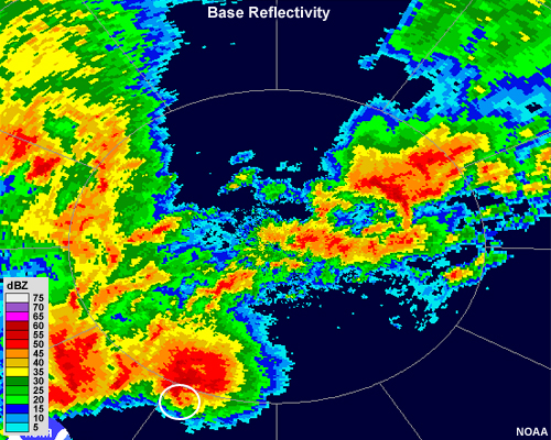
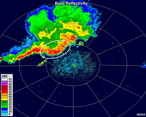
The most common type of radar product is called "base reflectivity." It is constructed by assigning a magnitude related to the amount of scattering that occurs from a target. In this image, the reflectivity in the center is "ground clutter"energy received from objects near the ground such as trees, buildings, or particulate matter in the air. The band of high reflectivity north of the ground clutter represents the precipitation intensity. The position of the precipitation is determined from two factors:
- Elevation angle of the antenna (how high the radar beam is pointing)
- Time it takes for the electromagnetic pulse to return to the radar
When looped together, these images give important information about the motion of precipitating regions.
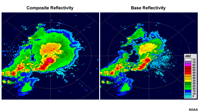
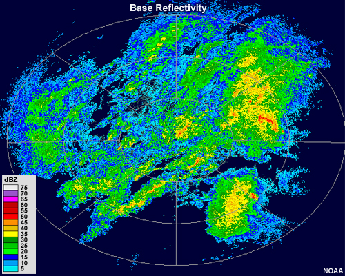
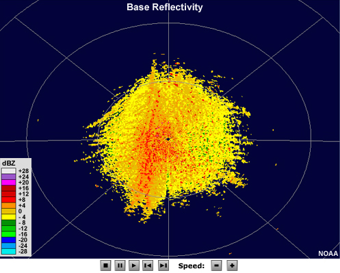
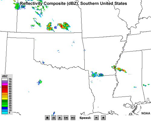
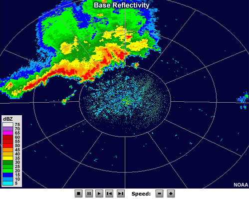
Another common display is "composite reflectivity," which shows the maximum dBZ in a given vertical column for all columns in the radar's range. Consequently, it gives a plan view of the most intense portions of a precipitating system regardless of its altitude. Composite reflectivity is very useful for noting heavy precipitation cores at mid-levels and for viewing the areal extent of precipitation at middle and upper levels. However, some of this precipitation may evaporate before it reaches the ground. To correctly use composite reflectivity you need to understand weather radar scanning geometry and also the typical structure of the observed phenomenon.
Velocity Products
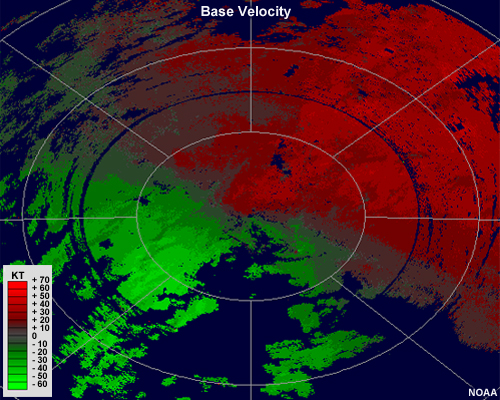
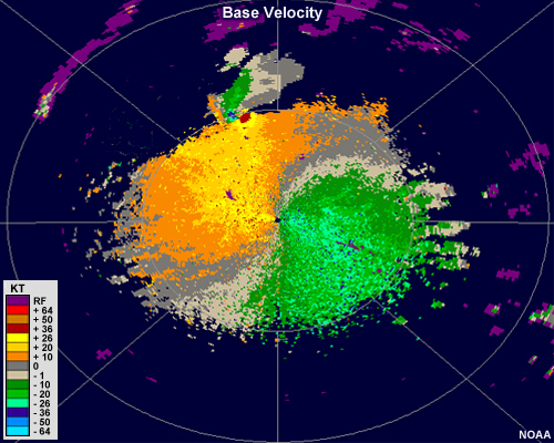
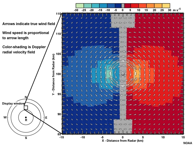
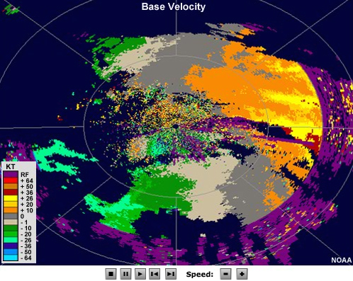
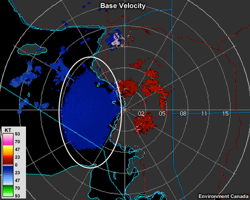
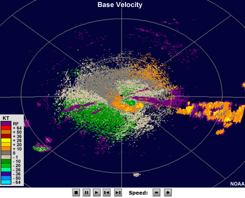
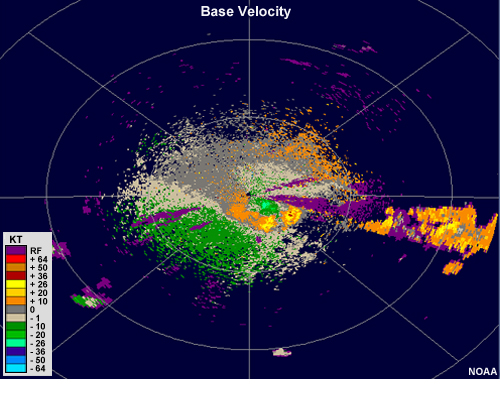
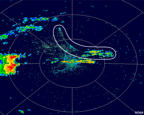
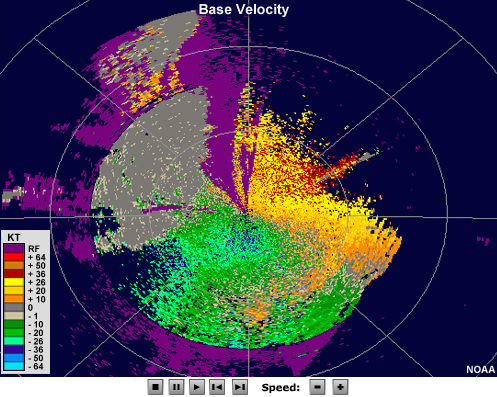
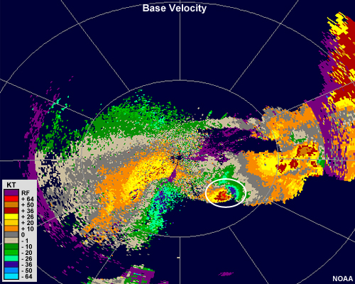
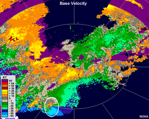
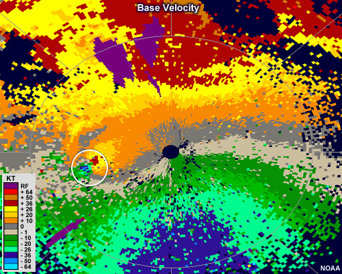
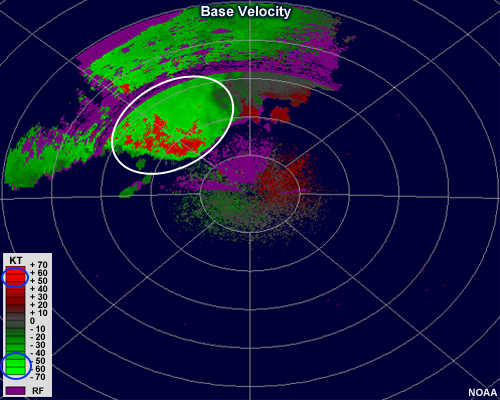
Base radial velocity images provide information about wind speed and direction. These are determined by whether a target is moving toward or away from the radar along a radial direction. In this example, warm colors (reds) indicate motions away from the radar and cool colors (greens) represent motion toward the radar. Targets that are stationary or moving perpendicular to the radar beam have no radial velocity and are colored gray.
These are the most common radar products and the ones we will focus on in this module. Other radar products, such as storm total precipitation and storm relative velocity, are also quite useful and may be explored here:
http://www.srh.noaa.gov/jetstream/doppler/baserefl.htm
Questions
Question 1
(Use the selection box to choose the answer that best completes the statement.)
Clear air is the correct answer. In clear air mode, the radar has longer to listen for echoes and provides a more detailed picture of the atmosphere.
Question 2
Which type(s) of radar can discriminate between precipitation types? (Choose the best answer.)
The correct answer is c.
Dual polarization radars transmit and receive data in the vertical direction as well as the horizontal, giving a more detailed picture of a target's shape and size. This allows a better discrimination between precipitation types. It is also possible for a phased array radar to have dual polarization, so in some cases answer b may also be correct.
Question 3
A NEXRAD WSR-88D radar can determine which of the following about the current weather? (Choose all that apply.)
The correct answers are a, c, and d.
NEXRAD WSR-88D radars cannot determine the phase of the precipitation (dual polarization radars can), and none of the radars discussed can determine the temperature of a target.
Question 4
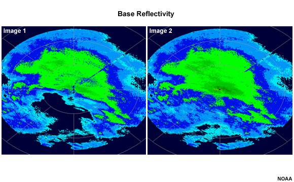
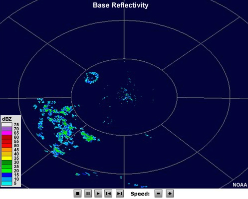
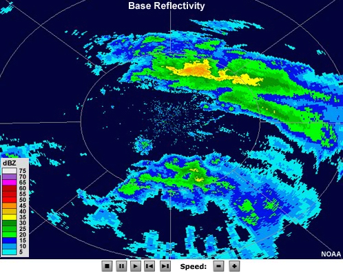
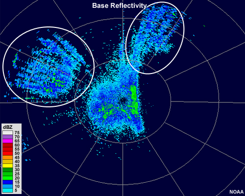
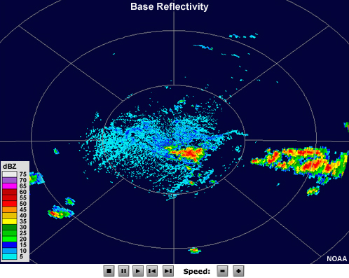
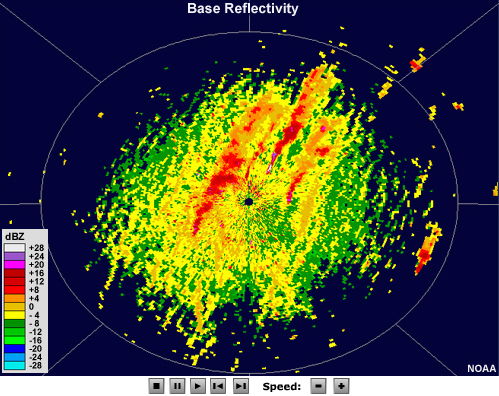
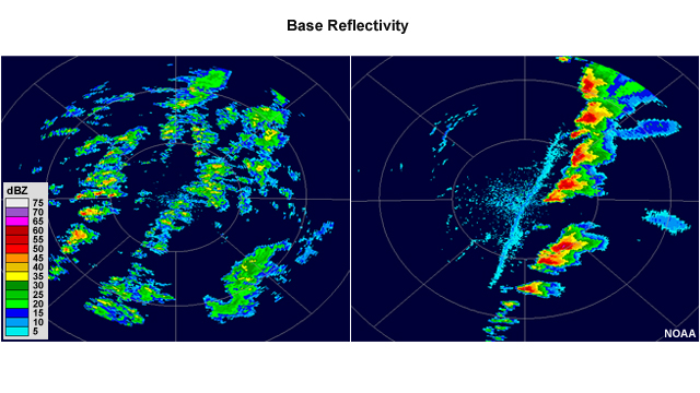
Which of these images shows composite reflectivity? Note: The images are from the same radar, date, and time. (Choose the best answer.)
The correct answer is b.
Image 2 shows composite reflectivity. Composite reflectivity shows the maximum dBZ in a given vertical column for all columns in the radar's range. This means that precipitation will appear more intense in some areas and will extend over a greater area than what is shown on base reflectivity. However, it may not correspond as well to what is happening on the ground.
Question 5
Which type(s) of radar can scan different sectors within its range and multiple sectors simultaneously? (Choose the best answer.)
The correct answer is b.
Because no mechanical rotation is involved, phased array radars can scan much faster and in any specific area that is desired.
Question 6
What is the cone of silence? (Choose the best answer.)
The correct answer is b.
The cone of silence is the volume left unscanned above the highest inclination angle beam.

Question 7
Match the radar product to the information that it displays. (Use the selection box to choose the best answer.)
The correct answers are shown above.
Question 8
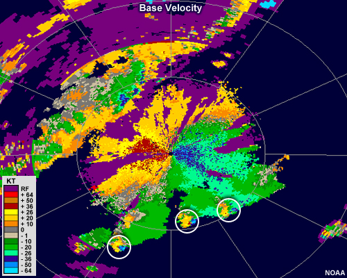
Match the base velocity image features with the location indicated by the letters. (Use the selection box to choose the best answer.)
The correct answers are shown above.
Limitations
The accuracy and usefulness of any forecasting toolnumerical model data, satellite imagery, or other data sourcesdepends on various factors that a forecaster needs to evaluate for each situation. The same is true for radar data. The radar processor operates on a number of assumptions that may not be met in many circumstances. In fact, it is possible for images to contain false readings.
A savvy forecaster needs to discriminate when radar data are valuable and when they contain erroneous data by keeping in mind the issues and assumptions discussed in this chapter.
Range Folding
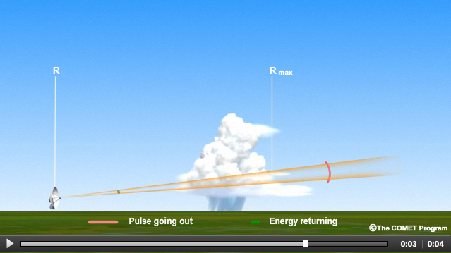
The time between pulses emitted by a radar must be long enough for any scattered energy from the first pulse to return before the radar has transmitted another pulse; otherwise, the radar will interpret the energy scatter from the original pulse as belonging to the second pulse. The maximum distance that a pulse can travel outward without this occurring is called the "maximum unambiguous range." For precipitation within the maximum unambiguous range, the radar pulses will go out and be scattered back to the radar before any additional pulses are emitted.
The location of the precipitation will then be plotted in the right location.
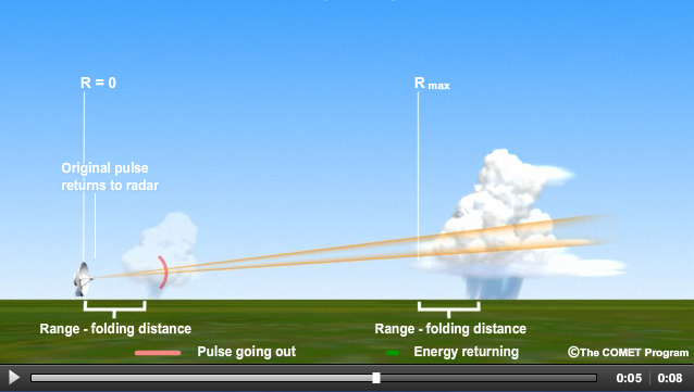
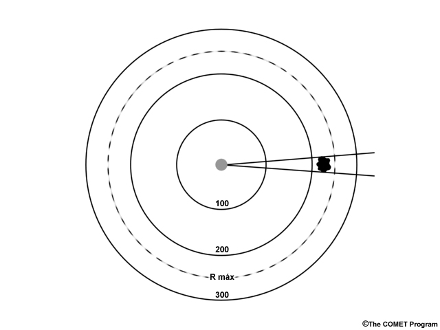
Now let's look at what happens when precipitation is located outside of the radar's maximum unambiguous range. After the pulse strikes the precipitation, the reflected portion is only able to make it part of the way back to the radar before a second pulse is transmitted. When pulse 1 finally does make it back to the radar, the radar interprets it as being a return from the second transmission, and it inaccurately places it closer to the radar. When they do appear, they often are elongated along the radial and may not look physically realistic.
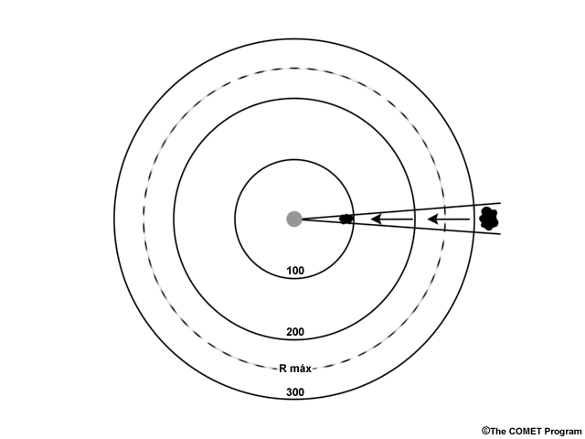
On a plan view image, the precipitating area will appear narrower and closer to the radar than it actually is, and it may look physically unrealistic. These types of radar echoes are sometimes termed "second trip" or "ghost" returns. The NWS often uses scanning strategies that have brief changes in the PRF (pulse repetition frequency) to help mitigate this problem.
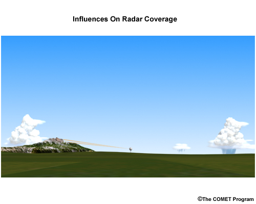
Viewing Angle
Viewing angle can also be an issue for targets far from the radar, depending on the type of precipitation and atmospheric conditions present. Convection can generally be viewed at some elevation by the radar except when a storm is very close within the cone of silence. Even then, the storm's low levels, where strong rotation and other hazards can still be detected, are somewhat observable. When precipitation is far away from the radar, even the lowest angle beam may overshoot important features. These types of problems become more pronounced for low-lying precipitation, as small areas close to the radar can be completely missed.
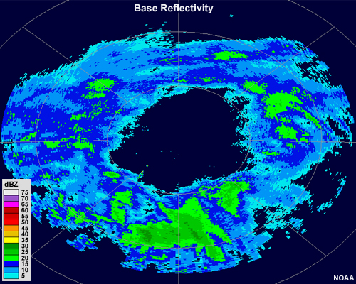
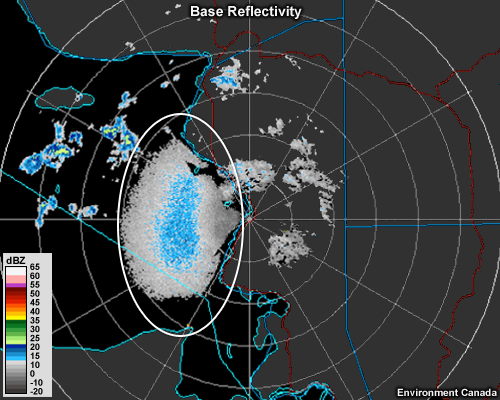
Here is an example in which none of the precipitation falling from a low, layered cloud reaches the ground. A donut shape appears on the radar return as the pulses do not encounter precipitation until they reach the cloud itself, pass through the precipitation, and then exit into the non-precipitating sky above.
Most of the time, fog goes undetected by radar because of its very low altitude and the small droplet sizes. But it may show up on radar in some cases where there is a thick layer of very dense fog and the radar beams bend toward the ground.
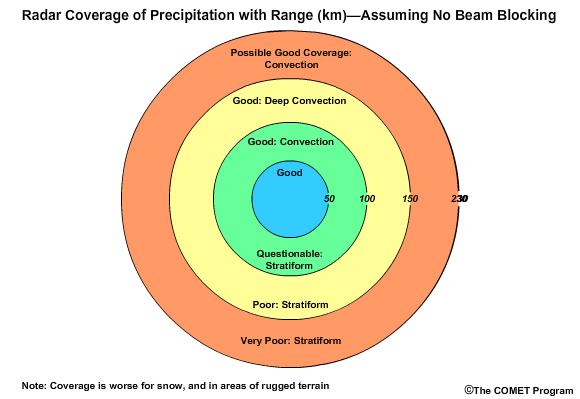
This graphic summarizes how well a NEXRAD WSR-88D radar can capture convective precipitation from tall clouds and stratiform precipitation from low, layered clouds.
Another problem with radar viewing angles is that of physical obstructions. It is sometimes unavoidable to site radars such that their low angle beams will not intercept the local topography.
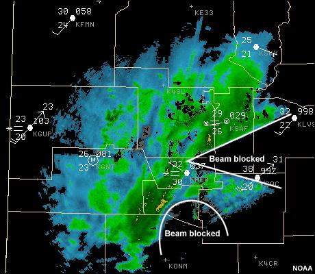
When this occurs, it is called "beam blocking," and low-angle beams will sometimes have a very short range. In cases of high mountains, many of the beams may be blocked.
Resolution
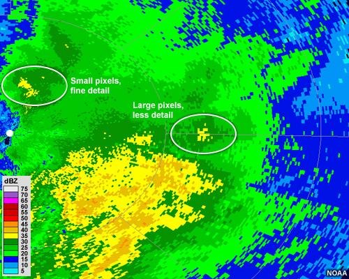
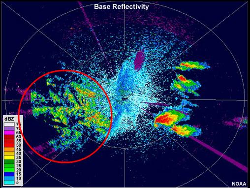
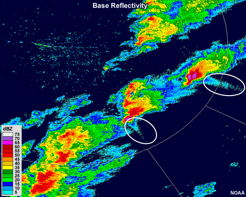
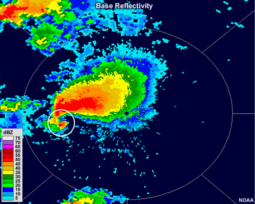
Because of the geometry of the radar beam, radar imagery inherently contains areas of varying resolution, which depends on the distance from the radar. Radar pulses broaden as they travel away from their source, creating ever larger sample volumes over which the reflectivity and other calculations are performed. This is evident in any radar image, as you can easily notice the relative small size of the pixels near the radar location and the larger size of the ones near the edge of the radar's range.
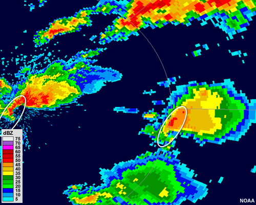
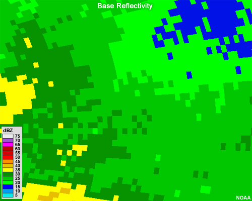
This poses some limitations when examining weather phenomena that are far away from the radar. Small but important features may not be observable as they will be averaged over an area that is larger than they are. For example, the thunderstorm nearest the radar (on the left of the image) is captured in great detail, especially its hook echo. The storm to the right looks similar, but the larger pixels don't allow us to pinpoint features as well as we can with the closer storm.
Processor Assumptions
The calculations for radar reflectivity and other variables are based on five main assumptions about the radar beam, the targets, and the atmosphere:
- The beam travels at the original inclination angle.
- The targets absorb very little of the radar's electromagnetic energy.
- Target particles are small, homogeneous precipitation spheres with diameters much smaller than the radar's wavelength.
- All targets are either liquid or frozen, but not a mixture.
- Targets are uniformly distributed throughout the sample volume.
Angle
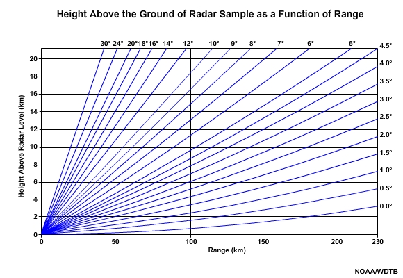
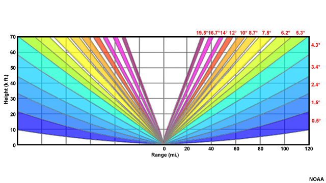
The first assumption is that the radar beam continues to travel through the atmosphere at its original inclination angle setting. As discussed before, most weather radars emit pulses at various elevation angles, ranging between the base scan of 0.5° and 19.5°. Under standard atmospheric conditions (that is, temperature and moisture both decrease with height in the troposphere), the beams will travel along paths that look like this.
Note that the height of each beam path increases as the beam travels farther away from the radar. This is because of the curvature of the earth. Deviations from these paths may occur depending on the refractive index of the air, which dictates whether electromagnetic waves will refract (that is, bend) when they pass from one material to another. When either a temperature inversion or sharp, vertical moisture gradient is present in the lower troposphere, the refractive index can change with height, essentially bending the radar beam path.
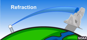
Under normal atmospheric conditions, a radar beam's curvature is slightly less than the earth's curvature.
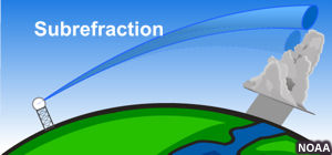
When the radar beam refracts (bends) less than it would under standard atmospheric conditions, it is called "subrefraction." When this occurs, the radar beam is more likely to overshoot areas of interest, and it will exit through the top of any precipitating area more quickly.
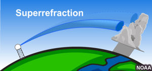
When the beam refracts more than the standard, it is called "superrefraction." In some cases, superrefraction can be so severe that radar pulses intercept the ground or become trapped, which is also known as "ducting." Superrefraction more commonly impacts radar imagery than subrefraction. When superrefraction occurs, the radar beam will bend downward and remain within a precipitating area longer. This can increase the radar's usefulness in examining precipitation that is far away, but may result in exceeding the maximum unambiguous range.
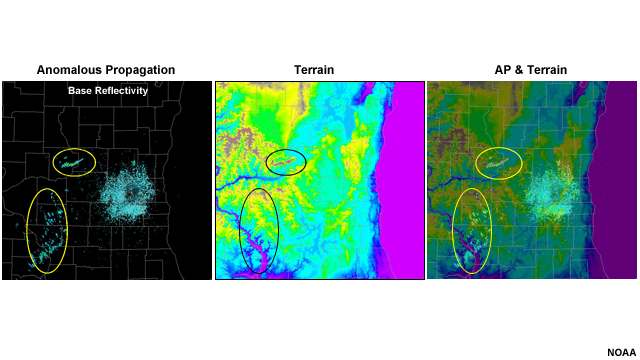
Additionally, the beam may intercept ground targets, creating confusing clutter on radar images. This is commonly called "anomalous propagation." In this example, the radar beams superrefracted enough that they intercepted some local topography that was about 50 km (30 mi) from the radar.
Superrefraction occurs mainly under the following conditions:
- Nocturnal radiation causing a temperature inversion near the ground and a sharp decrease in moisture with height
- A flow of warm, moist air over cooler surfaces, especially water
- A downdraft cooling the area underneath a thunderstorm, resulting in a temperature inversion in the lower troposphere. This is infrequent but can be very important because of its proximity to the storm.
Attenuation
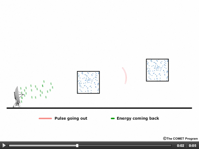
The second assumption is that attenuation due to absorption of electromagnetic energy by the targets is negligible. The amount of attenuation that can occur depends strongly on the intensity of precipitation and the wavelength of the pulses transmitted by the radar. In this illustration, you can see that most of the radar's energy is absorbed by the particles in the closest box, so the strongest returns would be from that area, rather than from the more distant boxeven though it has about the same number of targets.
Consider a situation in which an intense thunderstorm is close to the radar. Attenuation occurring in the heavy precipitation core of the closest storm can cause precipitating areas downrange to appear less intense. In severe cases of attenuation, some precipitation occurring downrange may not be displayed in the image at all.
In this example from a 5-centimeter (5-cm) wavelength airport Doppler weather radar, a line of thunderstorms is approaching the radar in the first image. When the strongest part of the storm passes overhead, attenuation becomes apparent in the middle image. Reflectivity values are especially reduced to the north and south, where the most intense precipitation aligns with the beam. In the last image, after the most intense precipitation moves past the radar, we can again see the rest of the storm structure. Generally, attenuation will increase as radar pulses travel through increasing amounts of precipitation.
Ten-centimeter (10-cm) wavelength radars, like those in the NEXRAD WSR-88D system, experience little attenuationthat is one of the reasons that wavelength was chosen for the system. In heavy precipitation, 3-cm and 5-cm wavelength radars, usually found in mobile platforms, airport surveillance and military applications, can suffer attenuation losses as much as 100 times higher than those experienced by a 10-cm radar. Nonetheless, this phenomenon may still pose problems for 10-cm radars if very heavy precipitation occurs over large areas close to the radar.
Homogeneity
A third assumption is that all target particles are small, homogenous spheres of precipitation that have diameters much smaller than the radar's wavelength.
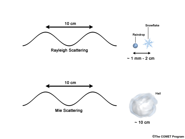
When the size of the particle is much less than the wavelength of the radar, a nearly linear relationship (called the "Rayleigh scattering regime") exists for the amount of scattering produced. This applies to most precipitation, as average raindrops range in size from about 1 mm to 4 mm and snowflakes are typically a bit larger. When the size of a particle is about the same as, or larger than, the radar wavelength, the scattering produced by particles becomes more complicated and falls under the "Mie scattering regime."
Because the radar equations are based on Rayleigh scattering approximations, any large targets (for example, hailstones, birds, some insects) will result in errors in scattering calculations and therefore reflectivity values. Furthermore, scattering calculations assume that the targets are spheres while birds, insects, and many hailstones are not. Therefore, reflectivity values from large targets should not be taken to be representative of their size.
Phase
Radar equations also assume that precipitation particles are all the same phase, but that is often not the case. Because ice and water have different structures and temperatures, ice does not scatter energy as effectively as water and returns about 7 dBZ weaker echoes than water droplets of the same size. Since the reflectivity equations assume that all particles are either ice or water, the true reflectivity value will be unknown. Without supporting temperature or sounding data, it is often quite difficult to determine whether an echo resulted from a region of snow, rain, or mixed precipitation.
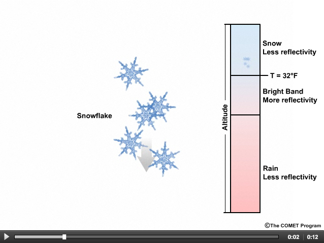
The melting level within a region of stratiform precipitation is often the exception to this rule, for a few reasons. First, snowflakes scatter less energy back to the radar than water. When snowflakes begin to melt on their way to the earth's surface, a liquid coating develops on their edges. This water coating often allows them to stick to nearby snowflakes, forming large aggregates of snow. The increase in size and in scattering due to the liquid coating means that reflectivity values increase within the melting layer. This is known as the radar bright band. The increase in reflectivity as snowflakes aggregate and start to melt can be as much as 15 dBZ.
As snow continues to melt, it collapses into more compact raindrops, which lowers the reflectivity values again. Additionally, the raindrops fall much faster than the snowflakes, reducing the number of targets in the area and further lowering reflectivity values underneath the bright band.
While this is easiest to see and understand in a cross-sectional view, it is sometimes apparent on base reflectivity scans as a ring or arc of higher reflectivity values around the radar site.
Uniformity
The radar reflectivity equation assumes that all particles are distributed evenly throughout the sample volume.
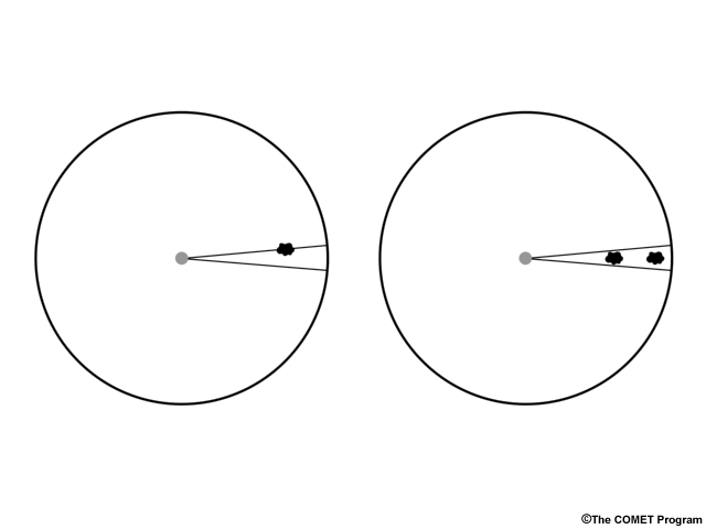
However, if small regions of precipitation fill only part of the beam, lower-than-actual reflectivity values will be displayed because the scattering is averaged over the entire width of the beam in that location. Precipitation that evenly fills the beam will produce a good reflectivity estimate.
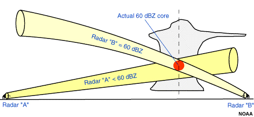
This is why two adjacent radars may come up with a different reflectivity value for the same location. For example, the area in red has a true reflectivity of 60 dBZ. Notice that only "Beam B" is completely filled with 60 dBZ, and would therefore assign a value of 60 dBZ to that location. "Beam A" is larger due to the longer range, and thus contains the 60 dBZ core plus weaker echoes surrounding it. This means that radar "A" will assign a reflectivity value less than 60 dBZ at the range indicated by the dotted line.
Questions
Question 1
Which of these images shows the area that is closer to the radar? (Choose the best answer.)
Image 1
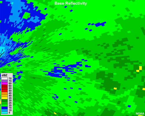
Image 2
The correct answer is a.
Image 1 shows data close to the radar. Since the beam broadens with increasing range from the radar, the pixels become larger with distance.
Question 2
For the following radar interpretation scenario, choose the aspect of radar geometry or operation that is probably causing the difficulty.
There is an intense thunderstorm containing large hail 16 km (10 mi) east of a military radar used to monitor aircraft. Another thunderstorm with reports of large hail is 40 km (25 mi) farther east. The forecaster on duty did not issue any statement or warning about the hail from the easternmost storm because reflectivity values for that storm were too low to indicate hail. What phenomenon likely caused this discrepancy? Explain.
(Type your answer in the box, then click Done.)
Attenuation is the likely cause of this scenario. When the radar beam had to pass through the first storm, some attenuation occurred such that a reduced amount of energy was available to scan the second, easternmost storm. This is probably what caused the lowered reflectivity values there.
Question 3
For the following radar interpretation scenario, choose the aspect of radar geometry or operation that is probably causing the difficulty.
You are walking home and it looks rainy. You call your friend who is on forecasting duty to ask if you will get soaked. She says that according to the reflectivity image, it is currently raining right where you are. You tell her that it is not raining anywhere that you can seethere are just some dark clouds above. What do you think caused this discrepancy? Explain.
(Type your answer in the box, then click Done.)
It is likely that your friend was looking at composite reflectivity instead of base reflectivity. Composite reflectivity shows the strongest reflectivity value within the radar range, and it is a mistake to interpret it as showing what is happening at the surface. If your friend was looking at a base reflectivity image, the precipitation probably evaporated before reaching the ground.
Question 4
What factors enhance the radar reflectivity around the melting level? (Choose all that apply.)
The correct answers are b and c.
Question 5
(Use the selection box to choose the best answer.)
If radar targets are similarly sized or larger in size than the wavelength of the pulses, Rayleigh scattering processes no longer apply and errors will be introduced in the reflectivity calculation.
Question 6
Why can two different radars obtain differing reflectivity values for the same location and time?
(Type your answer in the box, then click Done.)
This happens most often because the radars are different distances away from the location. Since the beam becomes larger as it travels away from the radar, the radar farthest away will be examining a larger volume than the other, resulting in two different reflectivity values.
Question 7
In which of the following instances would precipitation often go completely unobserved by NEXRAD WSR-88-D radar due to the geometry of the radar beam? (Choose all that apply.)
The correct answers are c and d.
Although the upper portions of a tall thunderstorm next to the radar would be in the cone of silence, the lower portions of the storm would be observable by low angle scans. A tall thunderstorm that was 50 km (31 mi) away from the radar would be well observed. A low, thin cloud far away from the radar would probably be under even the lowest 0.5° scan, and would go unnoticed. Beam blocking from a nearby mountain would probably obstruct views of rain on the other side.
Doppler Velocity Measurements
In this chapter we will look at how radial velocity is measured and calculated and how to analyze environmental wind fields and storm-scale circulations using velocity images.
Principles
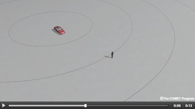
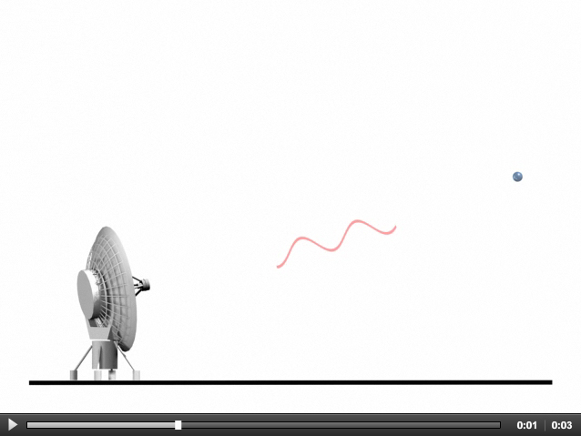
Pulse weather radars measure the wind field by harnessing the Doppler effect. This is the shift in wave frequency due to the movement of the wave source relative to an observer. You have probably noticed this at a race track, railroad crossing, or busy highway where the vehicles make a high-pitched sound that immediately changes to a lower pitch once they have passed you. For an example, play the animation.
While the driver hears only a constant sound, the observer hears a change in pitch. This happens because, as the source of the sound waves moves toward the observer, each wave takes slightly less time to reach the observer than the previous one, producing a higher frequency sound. When the source passes, each wave is emitted from farther away, resulting in a lower frequency sound.
Doppler Radars
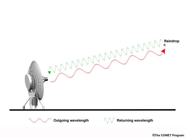
Because the same phenomenon occurs with electromagnetic waves, radars have been designed to measure this shift in frequency. The magnitude and direction of the shift give information about the motion of the target objects either toward or away from the radar. This measurement is called the "radial velocity."
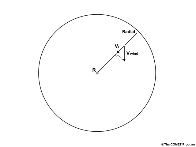
It is important to note that the radar can only tell whether a target is moving toward or away from it, and how fast it is doing so. The actual speed and direction of the wind will only be observed at points where the radar beam aligns perfectly parallel to a target's direction of travel. In all other instances, only the component of the target's motion that is parallel to the radar beam is measured and plotted as the radial velocity value.
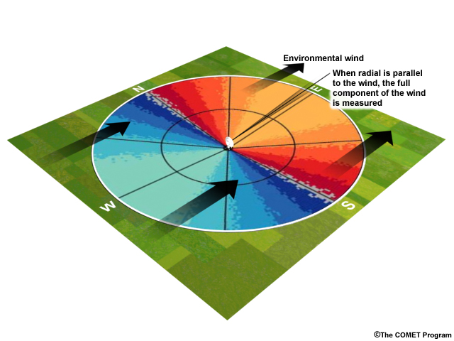
Let's look at a simple example in which the wind is blowing from the west at the same speed in all locations. When the radar beam is pointing directly to the east, the radar will measure the component of the wind that is parallel to the beam. In this case the radial velocity is the same as the environmental wind, which is displayed in a shade of red and orange to represent movement away from the radar.
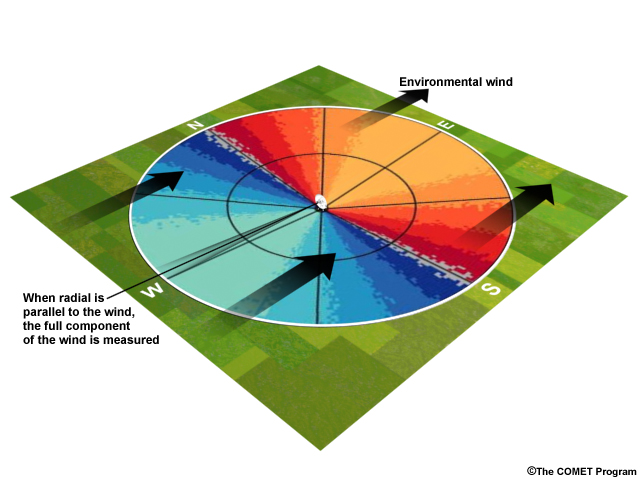
Similarly , when the radar beam points directly west, the radial velocity will be the same as the environmental wind, but will be displayed in green and blue shades to indicate movement toward the radar.
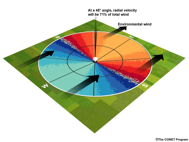
As the radar beam rotates, it will measure only the component of the wind that is parallel to it. In this case, at a 45° angle, it will measure about 71% of the total wind, so the reported radial velocity will be a lower speed than the actual environmental wind.
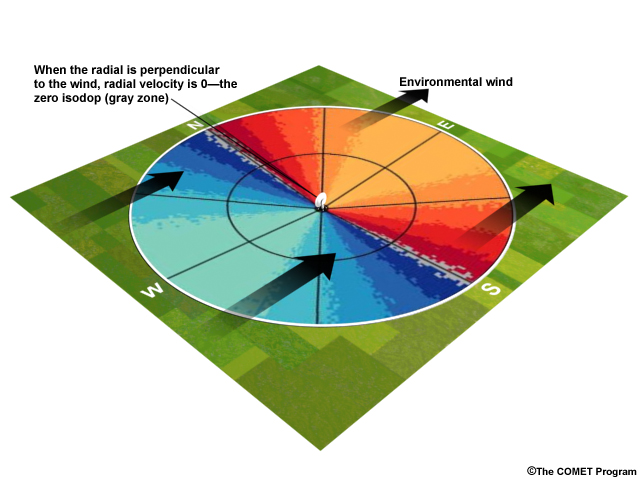
The radial velocity will be zero when the beam is perpendicular to the wind direction, as there is no parallel component.
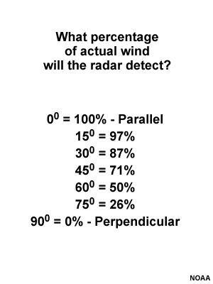
Note that the actual velocity of the wind did not change at any time or location in this example, just the angle at which it is viewed by the radar. This is why the speed of the wind can appear to greatly change over the viewing area on radial velocity images.
This may sound tricky at first, but with practice one can learn how to interpret these images and use them as a short-term diagnostic and forecasting tool.
Color Schemes
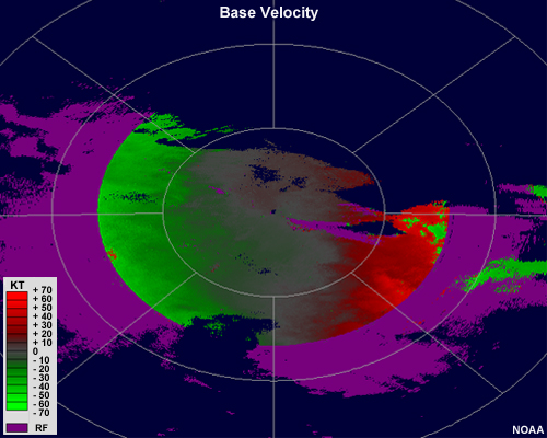
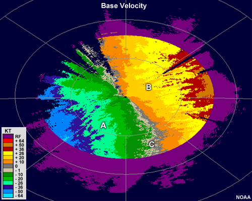
Most real-time NEXRAD WSR-88D radial velocity images use a scale in which shades of red represent motion away from the radar (positive values), and shades of green indicate motion toward the radar (negative values). Purple denotes range-folding (RF), which is when the return from a prior pulse is detected during the listening period for the current pulse, and the radar is unable to determine the wind's velocity.
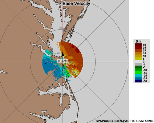
Other radar systems commonly use this color scheme, but some may use different colors. For example, the second velocity image includes yellows in the positive range and blues in the negative range. Forecasters can always expect the "cool colors" to be toward the radar and the "warm colors" to indicate motion away from the radar.
Large-Scale Wind Interpretation
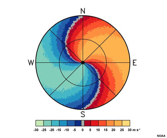
Let's begin with a simple exampleinterpreting a radial velocity image for a unidirectional wind field. First, remember that a radar pulse moves higher above the earth's surface as it travels from the radar. Thus, targets near the radar represent the low-level wind field, and targets farther away represent winds at higher altitudes.
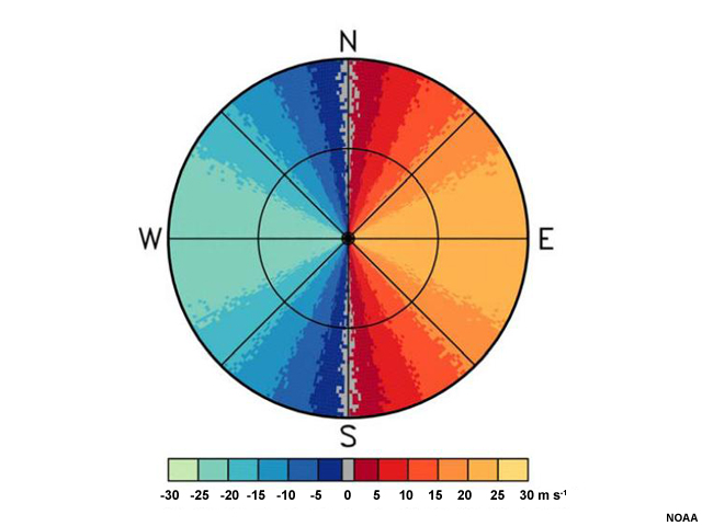
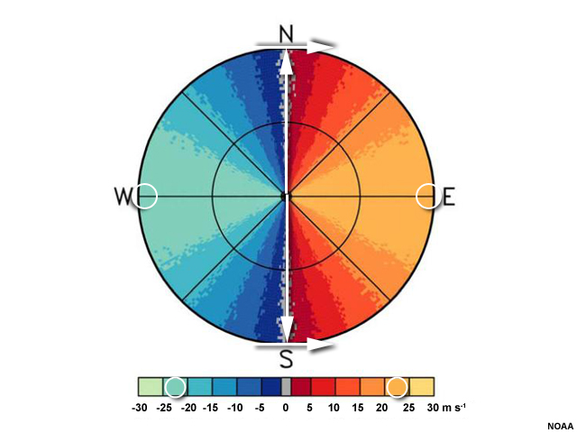
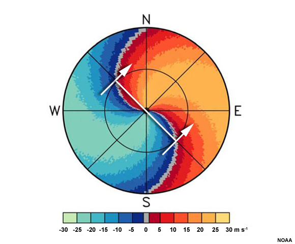
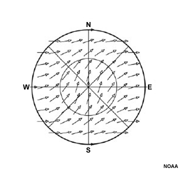
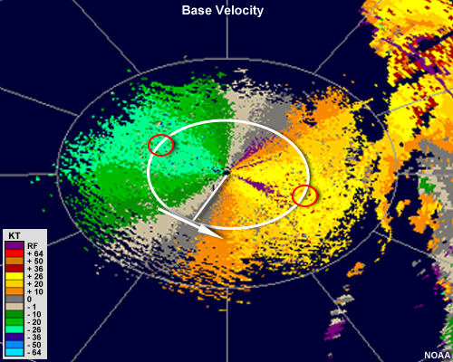
In this idealized base velocity image, winds on the left half are moving toward the radar. We often call these "inbound" winds. Winds on the right half of the image are all "outbound" winds. You can probably guess that the winds must have a westerly component. But is the true wind coming exactly from the west? How fast is it blowing at the surface? What about at higher heights?
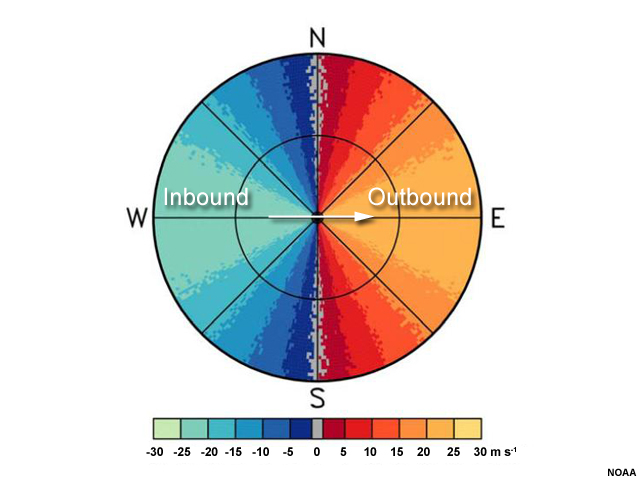
To determine the direction of the wind at the location of the radar, we simply need to find the closest measurement of the maximum inbound and maximum outbound radial velocities and connect them with a line.
To determine the wind speed and direction at a certain height away from the radar, we use the zero isodop.

An isodop is a line of constant Doppler velocity. The zero isodop is particularly useful because we know that the wind is perpendicular to the radar beam at any point along it. It could also mean that targets are stationary, but this is unlikely considering the fast winds we see near it.
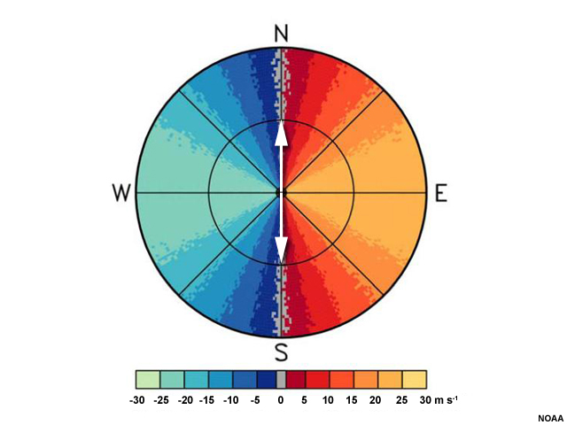
We begin by drawing an arrow from the radar's location to where the zero isodop intersects the specific height (i.e., the range) one wants to examine. In this case, let's figure out the wind direction at the first range ring from the radar. We draw an arrow from the radar location to where the zero isodop meets the range marker.
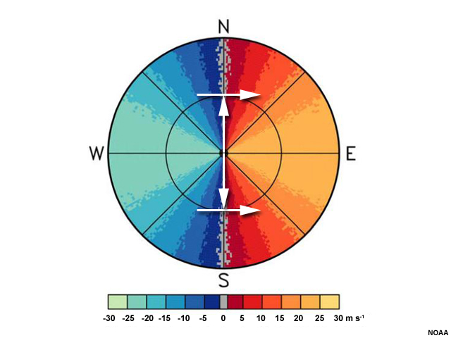
Next, we draw an arrow perpendicular to the first arrow we made, pointing from the inbound velocities toward the outbound ones. This will tell us the direction of the wind at that location.
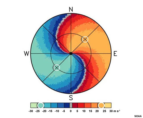
What is the maximum wind speed here? The easiest way to estimate the wind speed at a location is to find the maximum and minimum values that are anywhere along that same range ring from the radar.

In this case, we can see that there is a radial velocity maximum between 20 and 25 ms-1 and a minimum on the other side of -20 to -25 ms-1. Inherent in this method is an assumption that the winds are blowing about the same speed everywhere at a particular height.
We can perform both of these processes again to estimate the wind speed and direction at the edge of the radar's range. We draw a line from the radar location to where the zero isodop meets that range. Then, we draw our perpendicular arrow that represents the wind directiononce again, in this case, the direction is from the west. The wind speed can again be found by looking along that range for the maximum and minimum values. The maximum and minimum are again between 20 and 25 ms-1.
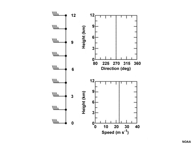
The winds in this example are westerly and the same magnitude everywhere. A sounding taken near a radar showing these radial velocities would have winds that look something like this.
Question
Here's a real example. What are the wind direction and speed at Portland? (Choose the best answer.)
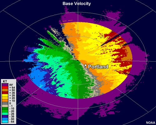
The correct answer is c.

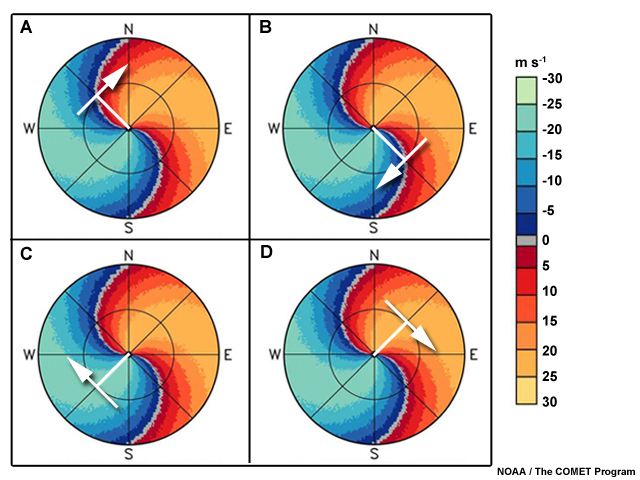
Directionally Sheared Winds
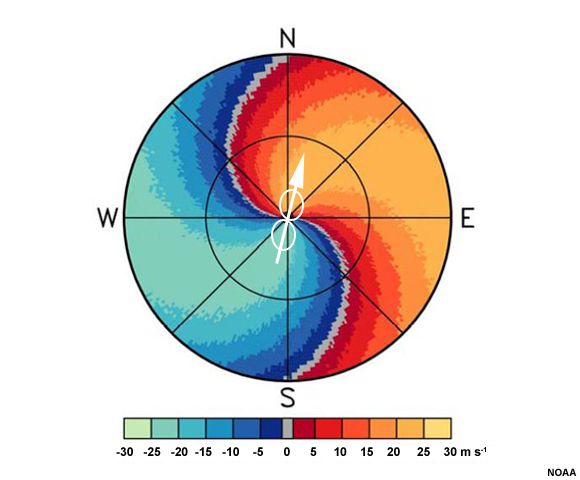
Of course, winds are rarely unidirectional, so let's look at a more complex case. At the location of the radar (and therefore near the surface), the maximum inbound velocity is just to the south, and the maximum outbound velocity is to the north. Connecting the inbound velocities to the outbound, we see that the wind is probably blowing from the south and perhaps slightly from the west. The speed is about 20 to 25 ms-1, as shown by the maximum and minimum values just next to the radar location.
Let's next determine the winds at the level of the first range ring.
Question 1
Which image best illustrates how to draw the radial and resulting wind direction at the level of the first range ring? (Choose the best answer.)
The correct answer is a.
Using the same methodology as the previous example, we first draw an arrow from the radar location to the point where the zero isodop intersects the range we are interested in. Then, we draw in an arrow perpendicular to it and pointing from the inbound to the outbound velocities. This is true for the opposite direction as well.
Question 2
What is the wind speed at the level of the first range ring? (Choose the best answer.)
The correct answer is d.
Examining along the rest of the range ring, we can see that the maximum values are 20 to 25 outbound and the same inbound.
Question 3
What is the wind speed and direction at the edge of the radar range? (Choose the best answer.)
The correct answer is b. Toggle to see an image that depicts what the resulting overall wind flow would look like if we estimated it for all locations.
Feedback

Overall Wind Flow
Real-world Examples
Example 1
Answer the questions to guide you through interpreting the winds in this radar image.
Roughly, from what direction is the wind blowing at the following levels: at the surface, at the location labeled "A" and the location labeled "B"? (Choose the best answer.)
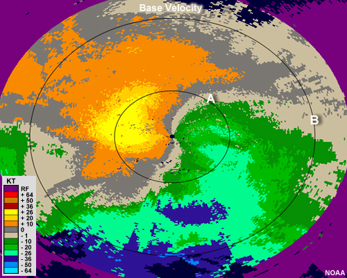
The correct answer is c.

If we draw the radials beginning at the radar and intersecting the zero isodop at these locations and then draw a perpendicular line to indicate the wind direction, we see that it is east at the surface, southeast at the location of the first range ring, and south at the location of the second range ring.
Example 2
What are the approximate wind speeds at the surface and location A, respectively? (Choose the best answer.)
The correct answer is c.
If we examine the color scale and look for the maximum and minimum near the surface, we see that the orange and dark green shades are touching the radar location, meaning the speed there is 10 knots. At the range indicated by point A, we can see a maximum of 26 knots and a minimum of negative 26 knots.
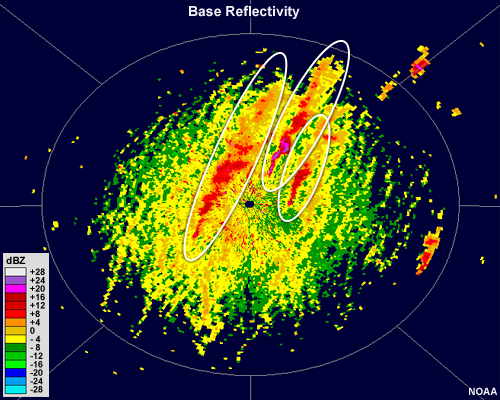
Maxima in Speed
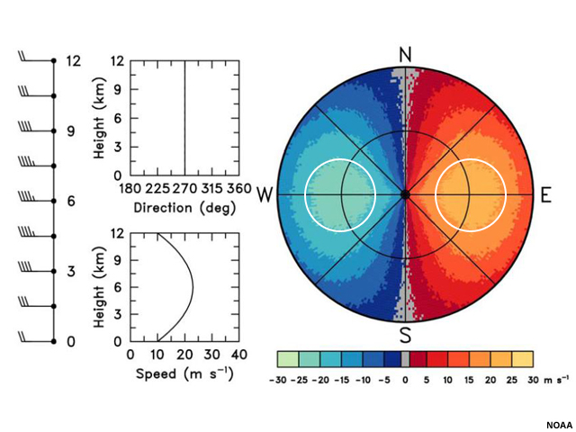
Wind speed generally tends to increase with height, but may not do so evenly. Sometimes, the polar jet stream will be sampled by radar, especially in winter, and low-level jets are routinely observed. In this idealized radial velocity image, the radial velocities show a maxima at the first range ring and above that wind speeds begin to decrease. This type of phenomena will typically show up on radial velocity images as two bull's-eyes that have closed isodops in some portion of the image.
Aliasing
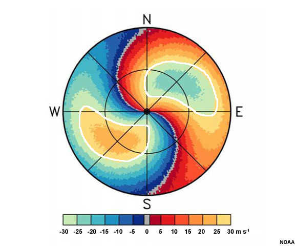
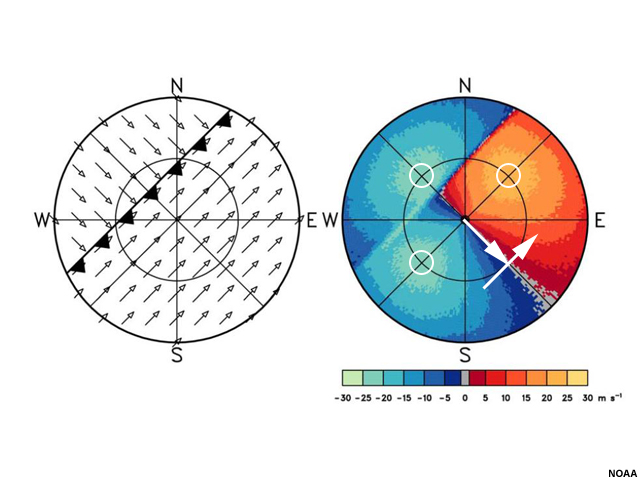
In some cases when very high wind speeds are present, such as when the radar samples strong jets or tropical cyclones, a radial velocity maximum or minimum will contain colors from the opposite wind direction in its center. Though one would normally conclude that the wind direction is somehow the opposite of the rest of the surrounding area and moving very fast, this is not correct. What we see here are in fact winds that change evenly from southerly at the surface to westerly at the edge of the radar's range that have a maximum speed at the level of the first range ring. The outlined areas in which the colors abruptly change to the opposite sign are a manifestation of the radar's maximum measurable velocity range. This phenomenon is known as aliasing or velocity folding.
Aliasing occurs when the radar's maximum unambiguous velocity is lower than the maximum velocity that is occurring. The maximum unambiguous velocity and maximum unambiguous range both depend on the pulse repetition frequency (PRF) but in opposite ways. This is a problem known as the "Doppler dilemma," in which a low PRF is desired for a large unambiguous range, but a high PRF is desired to observe high velocities.
When an environmental wind exceeds the maximum unambiguous velocity, the radar interprets it as a weaker wind of the opposite sign. The true environmental winds are offset by factors of 2*Vmax until they fall within the maximum unambiguous velocity range.
For example, if a radar's Vmax is 30 ms-1 and the environmental wind speed is 33 ms-1 away from the radar (positive and shaded in red-yellow), the radar will interpret this wind as being a 27 ms-1 inbound wind (negative and shaded in blue-green).

Here we have a thunderstorm complex containing strong winds. Some of the inbound winds are probably in excess of 70 kts. We can see aliasing where the red pixels are present within the large swath of strong green shades. Since there is no gradient or zero isodop present and the pixels abruptly change from red to green, aliasing is the likely cause.
Most NWS radars use some pattern of alternating high and low PRFs so that many of the aliased velocities and range-folded pixels can be removed or corrected by the software. Nonetheless, aliasing and range-folding remain complications to contend with, especially when using a shorter wavelength radar and in situations of very strong winds and wind shear, along boundaries, and in environments with significant clutter from non-meteorological targets.
Discontinuities
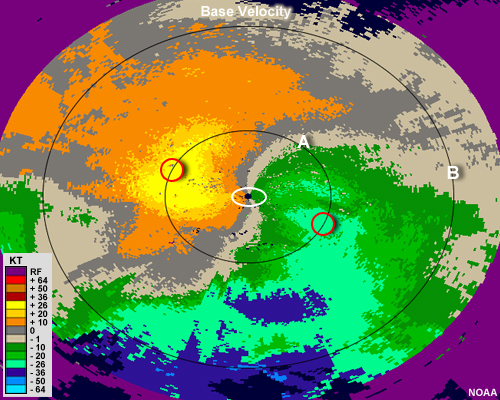
Here, we see that northwesterly flow associated with a cold front has a maximum near the level of the first range ring and is overtaking southwesterly flow that also has a maximum at the level of the first range ring.
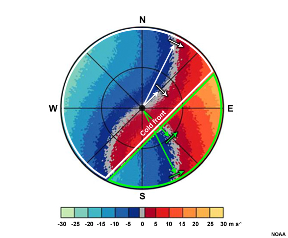
In some cases the radial velocity may look more like this. We can see that backing winds (turning counterclockwise with height) are occurring in the area outlined in white in the image, while the southeast portion (outlined in green) shows winds that appear to be veering (turning clockwise with height). Backing indicates cold air advection, while veering signals that warm air advection is occurring. This pattern would indicate a cold front moving into an area of warm flow with a southerly component, and we can see a sharp discontinuity that signifies the location of the front.
So far, we have examined large-scale interpretation of the environmental wind using radial velocity. Let's now take a look at some of the smaller scale circulations that can be diagnosed with radar.
Small-Scale Patterns

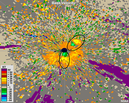
Earlier we saw the form a maximum in the overall environmental wind can take: a couplet of closed isodops with negative values on one side of the zero isodop and positive values on the other. This type of pattern also occurs for meso- and micro-scale phenomena, but for different reasons. There are two main types of small-scale couplets: ones indicating rotation and ones indicating convergence or divergence. A rotational couplet looks similar to the previous jet example, but usually at a much smaller scale embedded within the background flow.
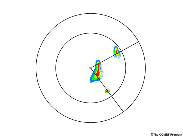
This image shows rotation occurring within a small portion of the radar's range. In this case, we see two sets of closed isodops. A line drawn from the radar location through the couplet will have the inbound velocity minimum to the left of the line and the outbound velocity maximum to the right.
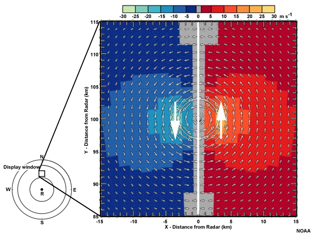
At such a small scale, this means that the winds are rotating rapidly in a counterclockwise fashion.
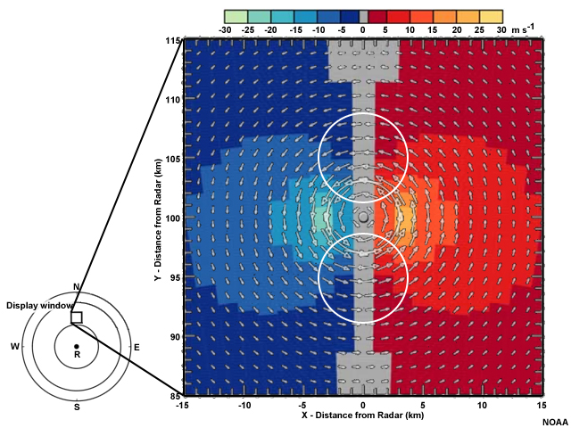
The easterly and westerly winds in this circulation are approximately the same strength as the northerly and southerly ones, but are not recorded as such because they are nearly perpendicular to the radial. Rotating updrafts in thunderstorms commonly produce this feature at low- to mid-levels of the troposphere.

In this example you can clearly see a well-defined couplet north of the radar. Drawing on the radial, we see that maximum inbound velocities are found to left while maximum outbound velocities are to the right. In this case, there is no zero isodop between the two maxima, which is often the case with thunderstorm environments. Often, the circulation is not strictly rotational, but also possesses a degree of convergence or other shear in the nearby storm environment.
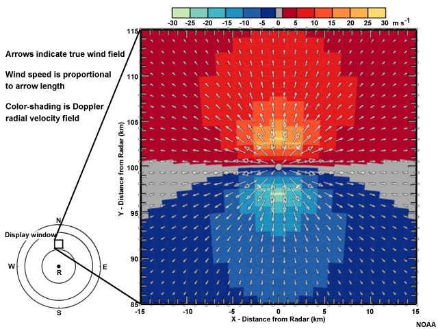
The other main type of couplet encountered in velocity images is one of convergence or divergence. It will look similar to other rotational couplets except the maxima will be oriented differently with respect to the radar beam.
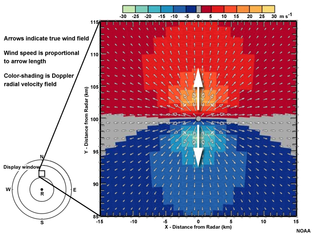
In this example, we see that a radar beam at this location would first see inbound velocities, quickly changing to outbound velocities farther downrange. This means that the winds are diverging away from the midpoint in this couplet. This can occur with strong thunderstorm downdrafts. A convergent couplet would look the same, except the positions of the outbound velocities would be found closer to the radar and the inbound ones farther away.
In this example, one divergent couplet is located northeast of the radar. We can see that the radar beam would first encounter outbound velocities, and then at the couplet, a maximum of inbound velocities followed quickly by a maximum of outbound velocities. A second divergent couplet from another microburst is south of the radar.
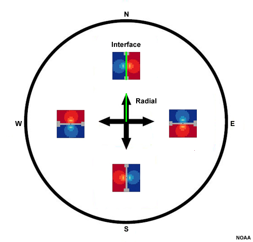
Another quick way to determine what type of couplet you're seeing is to draw a line that represents the interface between the inbound and outbound velocities. If the interface is parallel to a radar beam coming out to that point, then it is a rotational couplet.
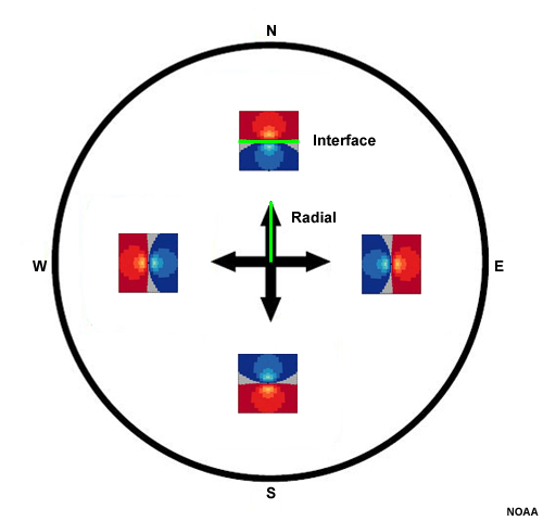
If the interface is perpendicular to it, then it is convergent or divergent. Many times, you will encounter some of both happening. We will examine some examples in the upcoming chapter that discusses convection.
Questions
Question 1
(Use the selection box to choose the best answer.)
Targets must have a component of motion toward or away from the radar to be measured.
Question 2
Estimate the wind speed and direction at the surface. (Choose the best answer.)

The correct answer is d.
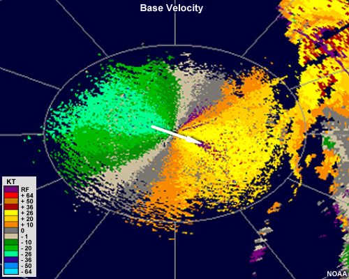
The light shades of green and orange touch the location of the radar. Drawing a line directly from the inbound velocities in green to the outbound velocities in orange at the location of the radar, we can see that the wind must be blowing from the northwest at approximately 20 to 26 knots.
Question 3
Estimate the wind speed and direction at the location of the white "X" in the image. (Choose the best answer.)

The correct answer is d.
Drawing a radial from the location of the radar out to the white X and then drawing a line perpendicularly from the inbound velocities there toward the outbound velocities, we can see that the wind must be blowing from the northwest. Its speed is approximately 20 to 26 knots, as evidenced by the maximum and minimum values at that same range.
Question 4
Match the couplet with the type of motion it is indicating. Assume that the couplets were associated with thunderstorms. Couplets are magnified to show detail. (Use the selection box to choose the best answer.)
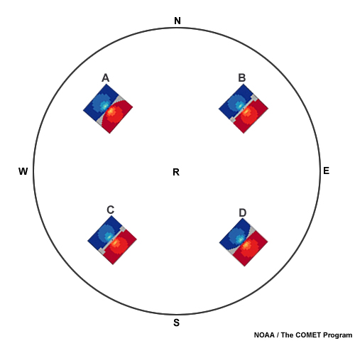
See feedback for each above.
Question 5
Aliasing occurs when the radial velocity exceeds the radar's maximum unambiguous velocity. (Choose the best answer.)
The correct answer is a.
Question 6
When aliasing occurs, the zero isodop appears between the aliased and unaliased regions, making it more difficult to determine what the winds are doing. (Choose the best answer.)
The correct answer is b.
As shown in this image, when velocities exceed the maximum unambiguous velocity, they are displayed as a wind of the opposite sign. A value of zero will not occur during this process, so aliased pixels will be located directly adjacent to usual velocity data without a zero isodop between the two.
Common Clear Air Phenomena
Radar can be used to identify a variety of fair weather phenomena. Often, the reasons we are able to get any radar returns at all is due to non-meteorological targets, such as dust, smoke, insects, and birds. Other times, anomalous propagation of radar beams is what allows us to see certain features. Commonly, it is a combination of both that reveals atmospheric processes.
Non-Meteorological Returns
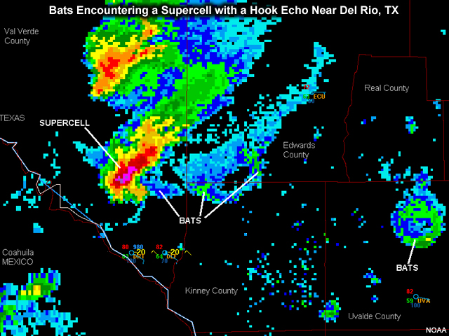
Radar targets can include all kinds of objects, ranging from live creatures, such as the returns from bats in this image, to particles released during military exercises. In this section we'll provide examples of a number of these radar echoes.
Biological Returns
Birds, bats, insects, and other airborne materials are often the only targets for radar pulses to intercept on clear days. Sometimes, they can produce their own unique signatures on radar. One of these is known as a "roost ring" or "bird burst." These are most easily diagnosed in a time series.
Birds often take flight near dawn, while bats leave their roosts near dusk (insects are also usually more active at night). Upon takeoff, these animals may quickly ascend several hundred feet as they spread across the area, forming a small ring that expands with time. Because most birds and bats fly relatively low to the ground, these types of echoes are generally only seen within about 30 nautical miles of the radar. Some larger birds, however, fly higher and may occasionally appear farther away.
Another way to distinguish whether what you're seeing is a mass of precipitation or some other kind of target is to look at its motion compared to the surroundings.
Look at this loop of radar reflectivity and then click the "Draw" tab. Then click the red pen to circle areas that might indicate radar echoes from non-meteorological targets. You may ignore any potential biological targets within any "ground clutter." After you are done drawing, click the feedback tab for comparison.
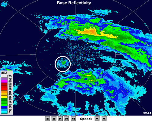
In this loop, a small area of what looks to be light precipitation rises suddenly to the southwest of the radar. It then begins to move rapidly northwest, counter to the rest of the precipitation that is moving to the east or southeast. This rapid initiation and travel in a different direction from the surrounding precipitation are two good clues that you may be looking at biological targets.
If we also look at a base velocity image, we can see that initially, the biological targets diverge from a single point and over time, head a different direction.
To summarize, here are a few things to keep in mind about diagnosing biological targets on radar:
- Reflectivities are low, usually <15 dBZ, for small birds and bats.
- Often a small patch will move against winds and/or surrounding precipitation areas.
- An expanding ring may signal takeoff en masse.
- Take note of the time of day and season. Mass exit of roosting areas is typical at sunrise (birds) and sunset (bats, insects), and migration is most common in spring and fall. However, there are numerous exceptions.
- Birds typically cause wind speed errors of 19-29 kt (10-15 m s-1); large insects might generate a bias as high as 12 kt (6 m s-1).
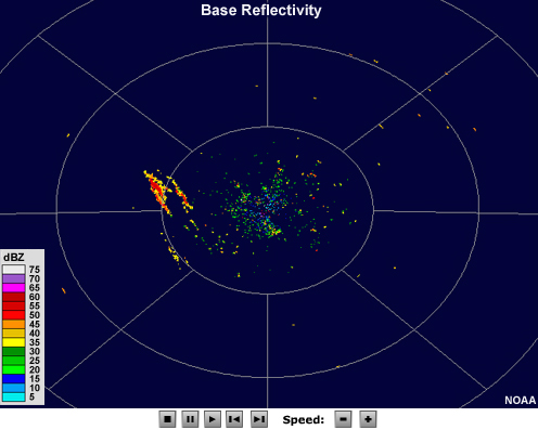
Anomalous Propagation
As we saw earlier, anomalous propagation (superrefraction) most commonly occurs when sharp inversions in the lower troposphere bend radar beams downward as they travel away from the radar. This phenomenon may cause a widespread cluttered appearance at the ground, or only certain features, such as local hilltops or buildings, may be intercepted. This image shows an example of anomalous propagation.
Here are a few key points to keep in mind about anomalous propagation echoes:
- When viewed as a time series, echoes will not change much over several frames. Some echoes may disappear or reappear, but will do so in mostly the same location.
- The targets' velocities in the suspected area will be at or nearly zero.
- Reflectivity values in areas of anomalous propagation are often erratic and do not resemble any usual precipitation patterns.
- Echoes may also be relatively weak and extend for great distances in a beamlike shape.
- Look at another nearby radar to help determine whether an echo is from precipitation.
- Look at recent satellite data to see if there are actually any clouds present.
- Look at the most recent local sounding to see if a sharp inversion is present.
- Look at a map of local topography to see if echoes are collocated with higher terrain.
Toggle between the loop of radar reflectivity and base velocity, then click "Draw" and use the red pen to outline any regions of anomalous propagation. After you are done drawing, click the feedback tab for comparison.
The area of anomalous propagation is circled in red. Radar reflectivity returns change only slightly in intensity over the duration of the loop, they do not move, and they do not look like usual precipitation patterns. The echoes in this area also show up very clearly with radial velocities of zero in the base velocity loop. The long purple beams are range-folded and likely a result of ducting and/or ground interference.
Sea Clutter
Reflectivity
Velocity
Sea clutter results from radar beams intersecting with waves and sea spray on lakes, seas, and oceans. This phenomenon occurs most often during times of rough seas and can be compounded when superrefraction occurs.
Usually , sea clutter has the following characteristics on radar:
- Low reflectivity values
- Usually present in only the lowest scans
- A fine, slightly grainy texture
- Echoes generally persist in their location and intensity
- Radial velocity shows prevailing wind direction, as waves and spray move with the wind
Smoke and Chaff
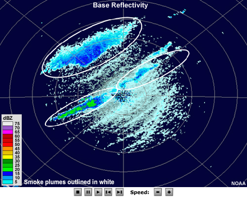
Smoke from wildfires or industrial sources can often show up on radar if it rises high enough into the troposphere. Often you can confirm that the echoes are from smoke plumes by looking at satellite data.
Usually , smoke has these characteristics on radar images:
- Low reflectivity (<20 dBZ)
- The echo elongates over time in the direction of the wind
- The echo will persist in the location of the source
- Radial velocity will indicate the prevailing wind direction and speed, as smoke particles act as tracers
A similar radar reflectivity return can occur when chaff has been released during nearby military exercises. Chaff is small, highly reflective particles that aircraft release to confuse other radar and targeting systems. These narrow echoes will travel in the same direction as the wind, and will not persist in a source location like smoke will. Chaff is most common near air bases and other military installations.
Other non-meteorological returns also occur and may be explored via these links:
Meteorological Returns
The radar's can also reveal a number of meteorological features produced by temperature and moisture gradients that can be precursors to precipitation events. We'll investigate some of those in this section.
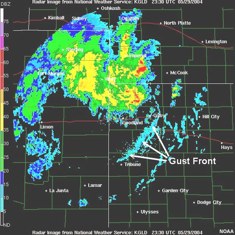
Fronts and Other Boundaries
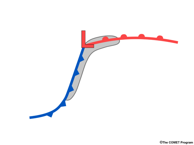
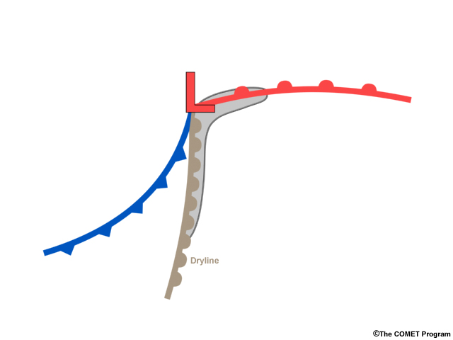
Frontal passages can be seen on radar even when no precipitation is present. The primary mechanisms responsible for this are insects and other particulate being concentrated due to convergence and turbulence along the front, and some degree of beam-bending due to density gradients along the boundary. Warm and cold fronts, drylines, outflow from thunderstorm downdrafts, and sea and lake breezes can all show up on radar when precipitation is not immediately nearby.
Most fronts and boundaries that lack precipitation have the following characteristics on radar:
- A very thin line of low reflectivity (<=15 dBZ), which is often called a "fine line." The line may appear as a narrow strip of enhanced reflectivity if the surroundings are significantly cluttered.
- An arc-shape to the fine line, which moves away from a recent thunderstorm in the case of outflow boundaries
- A distinct difference in wind direction behind and ahead of the front, if enough scatterers are present on both sides
Fronts often serve as lifting mechanisms and produce precipitation or thunderstorms later in the day, provided there is enough moisture ahead of the front. This is especially true if multiple boundaries intersect each other. These regions may also produce turbulent motions that should be monitored for aircraft concerns.
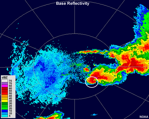
In this example, we can see a fine line of enhanced reflectivity when the loop begins in clear air mode. Thunderstorms begin to develop rapidly along this dryline and forecasters switch to precipitation mode accordingly.
Question
Reflectivity
Velocity
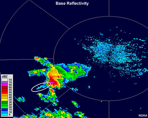
What type of front or boundary do you think we are seeing in these animations? (Choose the best answer.)
The correct answer is e.
This is a textbook example of an outflow boundary. We can see a very distinct ring of enhanced reflectivity emanating away from a cluster of thunderstorms just to the southeast of the radar. Additionally, we can see a signature of strong divergence in the location of the cluster of thunderstorms at the beginning of the animation (toggle below to see the couplet in a velocity image and an idealized representation).
Velocity
Idealized Couplet
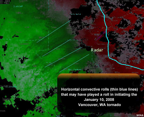
Horizontal Convective Rolls
Horizontal convective rolls are counter-rotating horizontal circulations within the boundary layer and are often a precursor to convective development. They usually appear on radar on mostly clear days with strong surface heating and a fairly steady wind direction. Insects and other particulates act as tracers of the roll circulations before clouds form, and birds are often present in these areas to feed on the concentrated insects.
You will usually see a large area of scattered low reflectivity returns close to the radar. Often, you will be able to discern several distinct lines or areas of enhanced reflectivity. Commonly, you may notice these features on radar:
- Evenly scattered amount of weak echo near the radar location
- Several lines of enhanced reflectivity, often appearing as ripples
Dust
During times of drought or in arid regions, great amounts of dust can be transported in the atmosphere. Dust storms can arise from several conditions, but often accompany thunderstorm outflow boundaries or strong synoptic frontal passages. This may or may not appear on radarit depends on how close the dust is to the radar location and how high it rises. Thus, situational awareness regarding hydrologic and soil conditions is necessary.
Some common characteristics of dust storms on radar include the following:
- Often associated with outflow boundaries and very strong synoptic fronts
- Can appear as a radar fine line that develops significant clutter behind it
- Generally low reflectivity values compared to precipitation
- Large dust particles will not rise as high as smaller ones, so reflectivity values within the dusty area will be highest near the surface
Questions
Question 1
Click the image below, watch the loop, then click "Draw" to use the pen tool to outline any fronts or boundaries you see in the still image from the loop.
A fine line of low radar reflectivity associated with a lake breeze advances to the southwest.
Question 2
Which of these phenomena is the radar detecting in this loop? (Choose the best answer.)
The correct answer is c.
The elongated echoes remain in the same source location while extending downwind with time.
Question 3
What phenomenon is the radar detecting in this loop? (Choose the best answer.)
Reflectivity
Velocity
The correct answer is b.
Superrefraction has likely bent these beams into the ground. This accounts for the velocities of zero on the base velocity images.
Question 4
Click the image below, watch the loop, then click "Draw" to use the pen tool to outline all areas which are likely to contain biological targets (aside from ground clutter).
The areas containing biological scatterers are outlined in white.
Question 5
What usually constitutes ground clutter that we often see near a radar? (Choose all that apply.)
The correct answers are a, b, c, and e.
Fog is not usually viewable by standard radar because of its very low height.
Question 6
Which of the following phenomena appears on radar as evenly scattered bands of weak reflectivity or ripples near the radar, especially during the afternoon? (Choose the best answer.)
The correct answer is c.
Horizontal convective rolls usually appear on radar on mostly clear days with strong surface heating and a fairly steady wind direction. Their circulations concentrate particulate matter and insects, making them visible to radar.
Convection
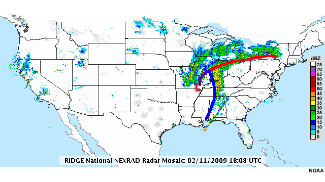
In this national reflectivity composite, there are at least two fronts present associated with precipitation. Depending on season and location, precipitation along these fronts may be either frozen or liquid, and it can often be difficult to distinguish between the two on radar. Convection, however, is usually easily distinguished by its high reflectivity values (>45 dBZ) and its initially cellular shape. In this chapter, we will look at features common to all thunderstorms as well as the typical locations, appearances, and radar signatures of three thunderstorm structures: ordinary thunderstorms, supercell thunderstorms and mesoscale convective systems.
Low-level Reflectivity Gradient
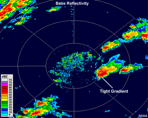
Most thunderstorm cells will have a central region, or core that exhibits strong reflectivity values. This core will usually be surrounded by lower reflectivity values. Tighter gradients of reflectivity between the edge of the cell and the core usually indicate a stronger storm.
The presence of a tight gradient indicates that large hail and/or heavy rainfall is sharply separated from the low-level updraft, which is the energy source of the storm.
For example, the lines of thunderstorms in the left panel are not as strong as the line of thunderstorms in the right panel, where we can see a very sharp change from almost no radar return to over 60 dBZ in the cores in some of the larger cells.
A forecaster can use this information as a guideline of general storm strength when initially assessing a storm situation.
Hail
Generally, the higher the reflectivity value found in a convective cell, the stronger the thunderstorm, and reflectivity values above about 60 dBZ usually indicate hail. Thus, a few of the storms in the left image may contain small hail, while nearly all of the storms in the right image probably contain hail, some of which is likely quite large. Keep in mind that any hail present in a sample volume may decrease in size via melting or sublimation during its descent, and that there is not a direct relationship between hail size and reflectivity value. Supporting information, such as the location of the freezing level and local spotter observations, can help determine what size hail is actually reaching the ground.
A particular signature to note for the presence of hail is called the Three Body Scatter Spike, or TBSS. A TBSS generally appears as a 10-30 km long (6-20 mi), low reflectivity (< 20 dBZ), mid-level echo "spike" that extends outward along a radar beam from a high reflectivity core. This echo spike is an artifact, formed when portions of the radar pulses are scattered to the ground and then reflected off the ground and back into the hail core, where they are interpreted by the radar as being from a location farther away.
A TBSS is a nearly certain indicator of large hail, as it generally occurs when the target size is close to the same as the wavelength of the radar pulse. It typically only occurs within the strong convection found in supercell thunderstorms.
Thunderstorm Structures
In the following sections, we will discuss how ordinary, or everyday, thunderstorms appear on radar. We will then examine the radar signatures of two specific thunderstorm structures that produce a large portion of severe weather: the supercell thunderstorm and the mesoscale convective system.
Ordinary Thunderstorms
The term "ordinary thunderstorms" refers to those everyday thunderstorms that have short lifetimeson the order of a few hours or less. They appear daily after sufficient surface heating has occurred. Some common locations where ordinary thunderstorms may be widespread are:
- The maritime, tropical airmasses that make up the "warm sector" of mid-latitude cyclones
- The back side of low pressure systems
- The edges of high pressure systems, and
- Along locally high terrain
These storms are usually not severe, but may contain small hail and gusty winds. In rare cases, otherwise ordinary thunderstorms can produce weak tornadoes, so any convection in the area should be monitored closely by radar.
On radar, ordinary thunderstorms generally develop quickly into small thunderstorm cores no larger than about 20 km (12 mi) in diameter. They have no characteristic shape and simply appear as small "blobs" with a small core of strong reflectivity values. Multiple cores may develop into larger clusters, but these too usually dissipate within a few hours.
To summarize, ordinary thunderstorms have the following characteristics:
- They are short-liveda few hours or less
- Generally are not severe
- On reflectivity images, they often appear as small, circle-shaped echoes that have a core of stronger reflectivity
- On velocity images, they have no consistent pattern, other than perhaps some divergence appearing near the end of their lifetime.
Supercell Thunderstorms
Supercell thunderstorms produce some of the most violent weather on earth. They are a unique form of single-celled convection that is defined by a rotating updraft.
Supercell thunderstorms usually develop just ahead of cold fronts and along the warm front close the center of low pressure.
They can also form along drylines. They typically last several hours, are prolific producers of large hail and tornadoes, and occasionally, damaging straight-line winds.
Supercells usually consist of a single cell of intense convection, usually about 30-60 km (20 to 40 mi) across the widest portion of the storm on radar. There are two hallmark signatures that characterize most supercell thunderstorms:
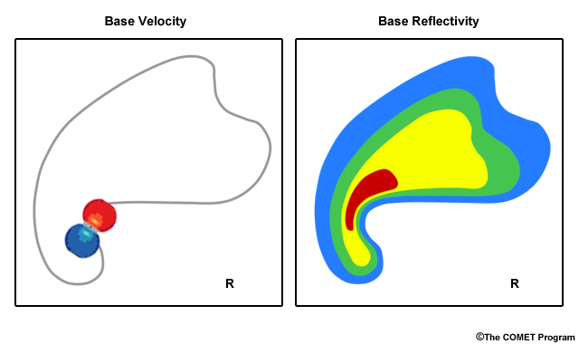
- A mesocyclone, which is a rotating updraft that displays as a rotational couplet and
- A hook echo, which is created by precipitation echoes wrapping around the mesocyclone.
Reflectivity
Velocity
In this example, the hook echo is rather broad, and the mesocyclone couplet is clear.
Reflectivity
Velocity
This hook echo is rather narrow and does not curve as much as a typical hook echo. Sometimes, hooks that look more like small appendages sticking out from the main convective core are referred to as "pendant" echoes. The mesocyclone couplet in this case is easy to discern and contains a significant amount of convergence as well.
Rotational signatures such as these may occur within some cells that comprise lines of convection, such as those that make up the leading portions of squall lines and some mesoscale convective systems. There, the rotation is usually smaller and weaker.
To summarize, supercells usually possess the following characteristics:
- Long-lived, lasting several hours
- Consist of a large, single cell of very strong convection that has a characteristic hook shape on radar reflectivity
- Have a rotating updraft that manifests as a rotational couplet on radial velocity
Question 1
Use the pen tool to circle the hook echo in this example.
Question 2
Use the pen tool to circle the mesocyclone couplet in this example.
Mesoscale Convective Systems
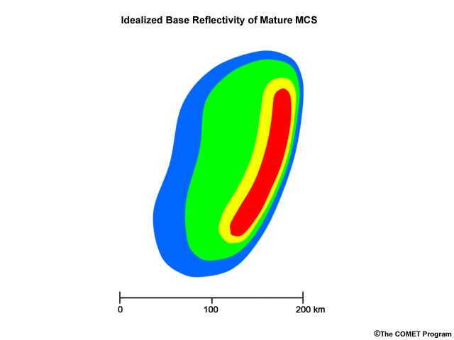
Mesoscale Convective Systems (or MCSs) are long-lived, organized systems that primarily occur during the warm season in mid-latitudes and the tropics. They often develop near warm and stationary fronts during the overnight hours in mid-latitudes, or in association with monsoonal circulations, easterly waves, and the ITCZ in the tropics.
MCSs commonly consist of a leading convective line, followed by a more expansive region of less intense and widespread precipitation. In some cases, a zone of weaker reflectivity will exist between the two areas.
Because of their large size and longevity, MCSs provide much of the summertime rainfall to the Great Plains and Midwest. They also generate a significant proportion of damaging wind events in the U.S. each year.
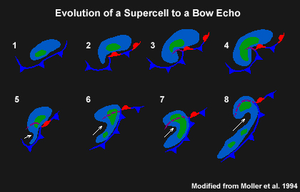
One of the most prominent features of many MCSs is the bow echo, which refers to a portion of a high reflectivity area that "bows " out ahead of the rest of the storm. Bowing is usually caused by a strong localized downdraft or sometimes a more organized, system-wide channel of air that flows from the back of the storm toward the front. These forces essentially "push" the leading convection ahead of the rest of the storm, forming a bowed segment.
In this loop, we can see how the bow develops quite rapidly.
Associated velocity images usually show very high radial velocities in the direction of motion of the bow. In this case, the velocities are so high that they exceeded the maximum unambiguous velocity and are aliased to be outbound rather than inbound. It is in this region of the MCS that damaging winds most commonly reach the surface.
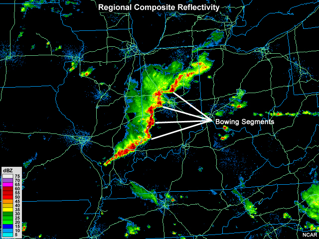
Bow echoes may also occur on smaller scales, and several may develop adjacent to each other within a single line of convection.
Bowing segments may also be found within more ordinary lines of convection and in association with some supercells. Forecasters should pay special attention to MCSs and other segments of storms that exhibit any bow echo characteristics.
To summarize, MCSs often possess the following characteristics:
- Long-lived, usually several hours or more
- Often consist of a leading line of strong convection and a trailing region of widespread, moderate precipitation
- May contain bow-shaped segments of intense precipitation within the leading convection
- May also contain damaging straight-line winds, especially just behind a bow echo, if it is present
To find out more about MCSs and their other associated radar signatures, please visit these other modules by COMET:
Questions
Question 1
What reflectivity value is a general threshold that indicates hail? (Choose the best answer.)
The correct answer is c.
Question 2
What type of thunderstorm organization typically lasts the longest? (Choose the best answer.)
The correct answer is b.
Question 3
What radar signature typically indicates that strong, straight-line winds may be occurring? (Choose the best answer.)
The correct answer is b.
The bow echo forms as strong winds from behind push the convective line into an arc or bow shape.
Question 4
Click image to open, then drag and drop circles to indicate all of the rotational or divergent couplets you see in this image. Click "Done" for comparison.
Question 5
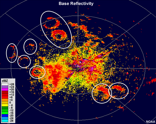
Drag and drop circles to indicate any hook echoes that you see in this image, then click "Done" for comparison.
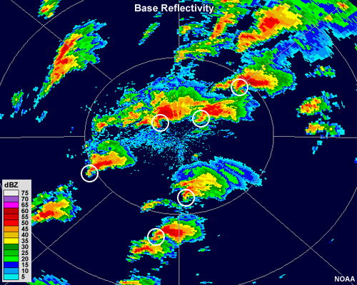
There are six pronounced hook echoes in this image, shown by the white circles. Other storms in the area were not exhibiting sharply pronounced hook echoes at the time of this image, but did either before or later in their evolution. Hooks on storms that are far from the radar may also be somewhat obscured due to decreased resolution or beam broadening.
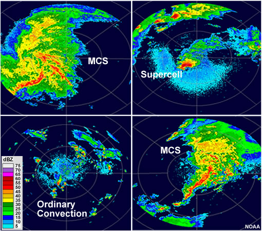
Question 6
Identify the storm type in each panel by dragging the labels to the appropriate position, then click "Done" for comparison.
Tropical Cyclones
Tropical cyclones develop in the tropics when the waters are at or near their warmest during the year. They are most common in the Atlantic Ocean from mid-summer to late fall. Typically, they travel on an east-to-west track that eventually turns poleward.
These systems can last as long as several weeks; produce strong storm surges; up to 50 cm ( 20 in) of rainfall a day; and contain winds of over 250 kph (155 mph) at their most severe.
Structure on Radar
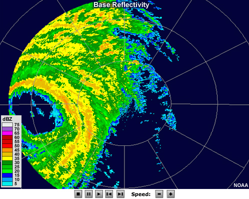
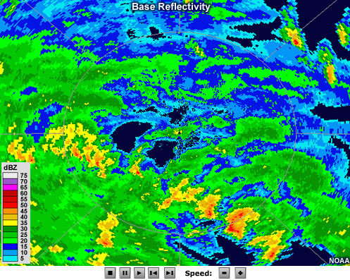
Tropical cyclones are easily recognized on radar. On reflectivity, they have three main noticeable features:
- The eye, which is a region that is nearly echo-free
- The eyewall, most often seen as a ring of high reflectivity surrounding the eye and frequently indicating some of the strongest convection in the system
- Spiral rainbands, which are narrow bands of intense rainfall that extend outward from the center of the storm
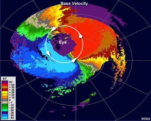
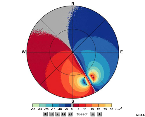
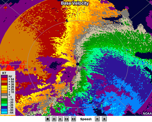
On velocity images, Northern Hemisphere tropical cyclones have a pattern that shows both their counterclockwise rotation and the speed maximum at low levels.
Here, we see that the radial velocity shows a symmetric pattern of counterclockwise flow, with the maximum wind speeds coinciding with the location of the eyewall. In the Northern Hemisphere, the velocities are slightly faster on the right-hand side with respect to the system's motion vector. This is because a tropical cyclone's forward motion and rotational motion are in the same direction on this side and add together. On the left-hand side, the rotational motion and forward motion are in opposing directions, resulting in lower speeds on that side.
Farther away from the radar, tropical cyclones often appear as a rotational couplet similar to that of a very large mesocyclone. Because of the very high wind speeds associated with tropical cyclones, aliasing may be present in some pixels of radial velocity images. In addition to this overall coupled appearance, storm-scale mesocyclones may be found within the stronger individual cells in some of the spiral rainbands.
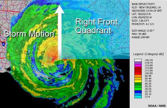
In the northern hemisphere, the occurrence of individual rotating cells is most common within the right front quadrant of hurricanes making landfall.
Reflectivity
Velocity
These cells can behave similarly to small supercells, and can produce weak to moderate tornadoes. It is often difficult to discern the small-scale rotation within individual cells in rainbands because of the already high velocities of the rotation of the hurricane itself. Aliasing may also cause some confusion. Rotational couplets in an environment like this may exhibit the usual inbound and outbound separation on either side of a radial drawn from the radar location and may contain some degree of convergence. In some cases, the couplet may appear more like a convergence signature than a rotational one.
To summarize, tropical cyclones on radar usually exhibit the following characteristics:
- Very low or no reflectivity within the eye
- An arc or ring of very high reflectivity in the location of the eyewall
- Additional narrow bands of high reflectivity emanating outward from the eyewall
- Storm-scale rotation within strong cells in the right front quadrant, especially within landfalling systems
Questions
Question 1
Tornadoes are most common within which quadrant of a tropical cyclone in the Northern Hemisphere with respect to the storm motion? (Choose the best answer.)
The correct answer is a.
Question 2
Drag and drop the feature labels over the area in which they are likely occurring, then click "Done" for comparison.
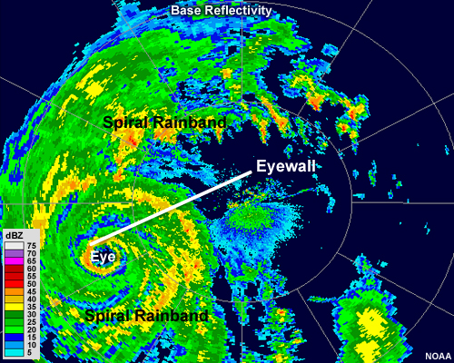
Question 3
The maximum wind speeds in a tropical cyclone are usually collocated with which of the following features? (Choose the best answer.)
The correct answer is b.
Question 4
Use the pen tool to outline those cells that are likely to have rotation, then click "Done" for comparison.
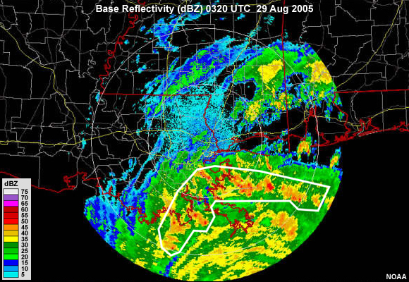
Winter Weather
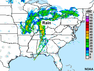
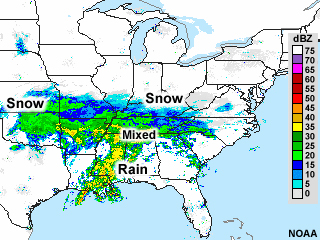
One of these mid-latitude cyclones produced rain, snow, and mixed precipitation. The other produced only rain. It can be difficult to tell using WSR-88D weather radar alone. This chapter discusses some general guidelines for estimating ice-phase precipitation versus liquid precipitation using radar.
Liquid versus Ice
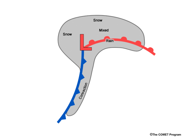
In many cases, the distribution of precipitation within a mid-latitude cyclone looks something like this. But that is not always the case, and using radar to determine where frozen precipitation exists is usually somewhat difficult.
Earlier we discussed that radar reflectivity was typically about 7 dBZ lower for a sphere of ice than a sphere of water due to ice scattering less energy than water. However, when one wants to determine where snow exists using non-dual-polarized radar, simply looking for regions of lower reflectivity is not a reliable method.
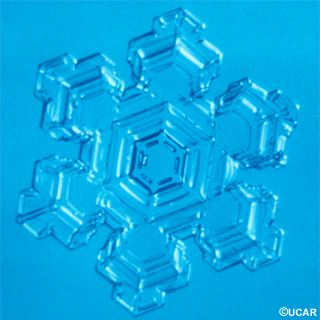
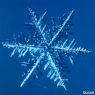
Because snowflakes can vary greatly in size and are often larger than raindrops, the reflectivity difference between ice and water is often reduced. In some cases of extremely large snowflakes, the reflectivity will be higher than in neighboring areas of rainfall.
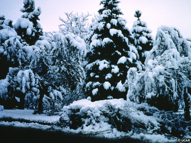
Also, the water content of the snow will impact the reflectivity value. The more water content the snowflakes have, the higher their reflectivity value. This is especially true of snowflakes that are melting, as they have a very reflective water coating on their edges while still retaining their large diameters.
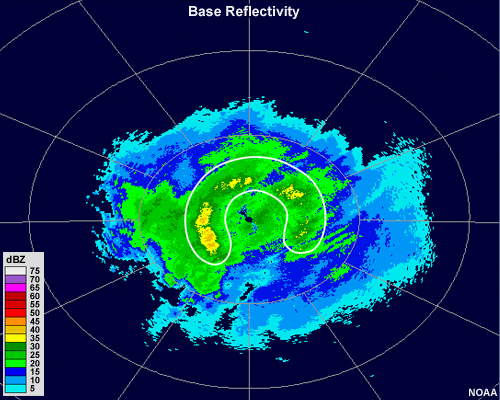
As discussed earlier, this can often produce enhanced reflectivity values at the melting level and appears as a bright band of higher values in an arc or ring around the radar location.
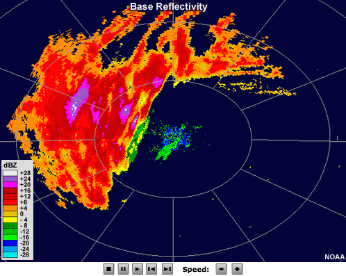
Dry, powdery snow often has quite low reflectivity values, and clear air mode may be used if it is the only precipitation in the area. Here we can see that maximum reflectivity values approach 30 dBZ, but only in a very small area. Most of this region of snow exhibits reflectivity values of 18 dBZ or less, and much of the region has values below 8 dBZ.
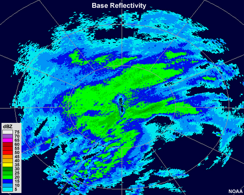
In this example, maximum reflectivity values are slightly higher, but the overall pattern is still one that shows the following:
- Gradual changes in reflectivity values
- Grainy texture
- Fuzzy echo edges
These are all characteristic of snow on radar but cannot be used to definitively determine what type of precipitation is occurring. They should be used as guidelines to make an initial assessment and to help determine precipitation type in regions that have few surface observations and/or no soundings available.
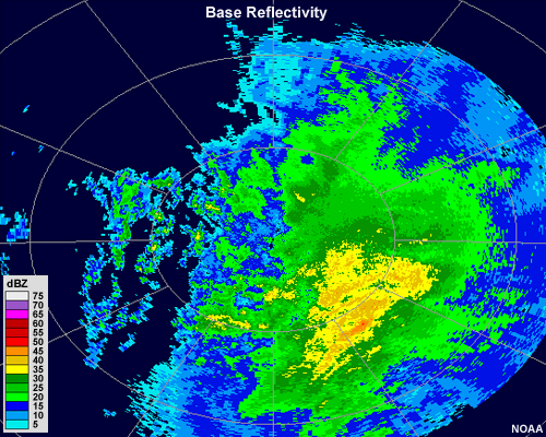
Wet, soggy snow will have much higher reflectivity values. Reflectivity values may even approach 45 dBZ. Snowfall with reflectivity values this high can often be confused for rainfall, but several of the indicators mentioned before are present: weak reflectivity gradients, a grainy texture, and somewhat fuzzy edges to the echo.
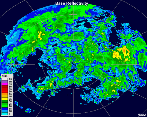
For comparison, a similar raining region of this mid-latitude cyclone looks like this. We can see that while the maximum reflectivity values are about the same as the snowfall loop, the reflectivity gradients are much sharper and the overall structure is more cellular in nature.
Snow Banding
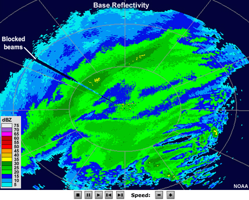
In the Northern Hemisphere, snow sometimes organizes into more intense banded patterns just north of the warm front and northwest of the low pressure center. These bands of snow can stand alone with no echo returns between them, but usually they occur as bands of enhanced reflectivity values among a generally consistent background level of snow. Snow banding is also common during lake effect and lake enhanced snow events.
Reflectivity
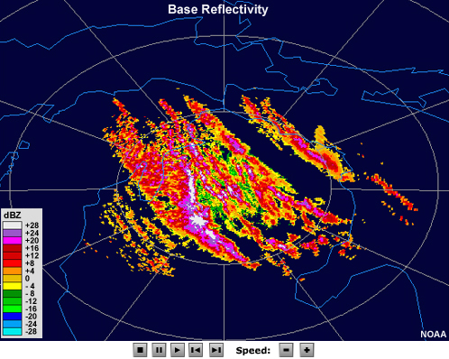
Velocity
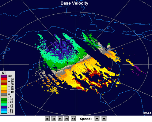
Lake effect snow usually takes the form of multiple narrow bands that are oriented parallel to the wind direction.
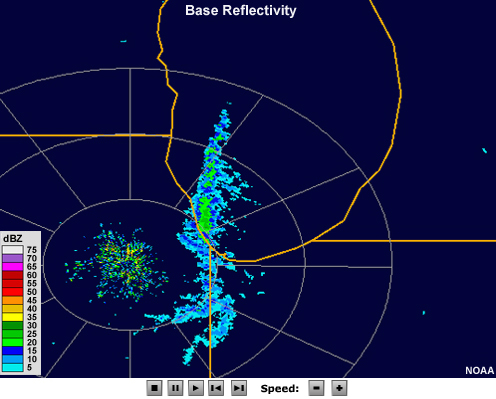
In some cases, a single, large band may set up along the center of the body of water.
To summarize, some useful indicators of whether radar is detecting rain or snow are the following:
- Snow usually contains very weak gradients in reflectivity value.
- An area of snow, especially dry snow, will have fuzzy edges instead of a distinct echo edge.
- An area of snow will often have a grainy, textured appearance.
- Snow may develop into bands of enhanced reflectivity, especially along the warm front, to the northwest of the low pressure center, and on the downwind side of lakes and other open water.
- Examine your local sounding and low-level temperature data to see what type of precipitation could develop.
Of course, dual-polarization radar data, when available, greatly enhances the ability to determine precipitation types.
Questions
Question 1
Use the white pen to outline the area in which it is likely snowing. Use the red pen to outline areas in which it is raining or precipitation is mixed, then click "Done" for comparison.
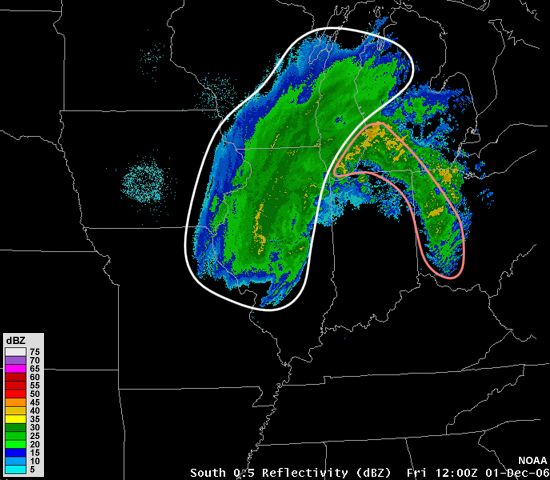
Question 2
Use the white pen to outline the area in which it is likely snowing. Use the red pen to outline areas in which it is raining or precipitation is mixed, then click "Done" for comparison.
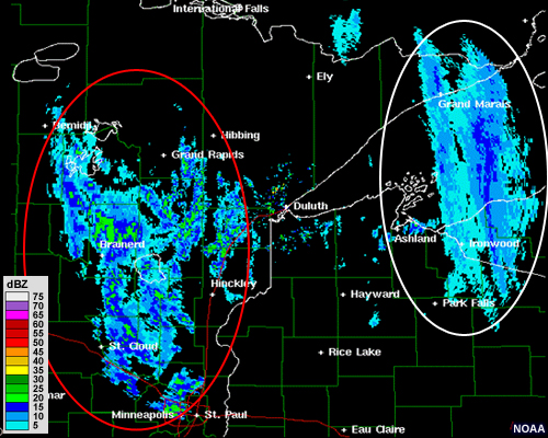
Notice the contrast between the grainy, fuzzy snow echo and the more cellular rain echo.
Question 3
Which of the following usually indicates that snow is occurring on a radar return? (Choose all that apply.)
The correct answers are b, c, and f.
Snow often appears as a moderate intensity echo that is widespread. It may also contain weak banded features. Snow also often possesses a "grainy" texture and has fuzzy, indistinct echo edges. Exceptionally wet, slushy snow may defy these rules.
Question 4
In which areas of a mid-latitude cyclone (in the Northern Hemisphere) is snow most likely to be found? (Choose all that apply.)
The correct answers are a and c.
Question 5
Which of the following are true regarding how lake effect snow appears on radar? (Choose all that apply.)
The correct answers are c and e.
Lake effect snow usually organizes into bands that are parallel to the direction of the wind and may also form a single, long band aligned with the center of a body of water.